
PENUGASAN
Contents
PENUGASAN#
from google.colab import drive
drive.mount('/content/drive')
KeyboardInterruptTraceback (most recent call last)
<ipython-input-1-d5df0069828e> in <module>
      1 from google.colab import drive
----> 2 drive.mount('/content/drive')

/usr/local/lib/python3.8/dist-packages/google/colab/drive.py in mount(mountpoint, force_remount, timeout_ms, readonly)
     98 def mount(mountpoint, force_remount=False, timeout_ms=120000, readonly=False):
     99   """Mount your Google Drive at the specified mountpoint path."""
--> 100   return _mount(
    101       mountpoint,
    102       force_remount=force_remount,

/usr/local/lib/python3.8/dist-packages/google/colab/drive.py in _mount(mountpoint, force_remount, timeout_ms, ephemeral, readonly)
    121       'TBE_EPHEM_CREDS_ADDR'] if ephemeral else _os.environ['TBE_CREDS_ADDR']
    122   if ephemeral:
--> 123     _message.blocking_request(
    124         'request_auth', request={'authType': 'dfs_ephemeral'}, timeout_sec=None)
    125

/usr/local/lib/python3.8/dist-packages/google/colab/_message.py in blocking_request(request_type, request, timeout_sec, parent)
    169   request_id = send_request(
    170       request_type, request, parent=parent, expect_reply=True)
--> 171   return read_reply_from_input(request_id, timeout_sec)

/usr/local/lib/python3.8/dist-packages/google/colab/_message.py in read_reply_from_input(message_id, timeout_sec)
     95     reply = _read_next_input_message()
     96     if reply == _NOT_READY or not isinstance(reply, dict):
---> 97       time.sleep(0.025)
     98       continue
     99     if (reply.get('type') == 'colab_reply' and

KeyboardInterrupt:
Tugas 1#
import pandas as pd

p=pd.read_csv('https://raw.githubusercontent.com/Rosita19/datamining/main/drug200.csv')
p.head()
| Age | Sex | BP | Cholesterol | Na_to_K | Drug | |
|---|---|---|---|---|---|---|
| 0 | 23 | F | HIGH | HIGH | 25.355 | DrugY |
| 1 | 47 | M | LOW | HIGH | 13.093 | drugC |
| 2 | 47 | M | LOW | HIGH | 10.114 | drugC |
| 3 | 28 | F | NORMAL | HIGH | 7.798 | drugX |
| 4 | 61 | F | LOW | HIGH | 18.043 | DrugY |
import math

print("Data Nominal \nTempat Lahir - Agama \nA=[Jombang, Islam] \nB=[Mojokerto, Islam] \nC=[Jombang, Kristen] \nD=[Jombang, Katolik]\n")
print("Data Binary \nGender - StatusKawin \nA=[1, 1] \nB=[1, 0] \nC=[1, 0] \nD=[0, 1]\n")
print("Data Numeric \nUmur - Berat badan \nA=[20, 45] \nB=[25, 60] \nC=[50, 55] \nD=[35, 70]\n")

#Nominal
#Tempat lahir - agama
A=['Jombang', 'Islam']
B=['Mojokerto', 'Islam']
C=['Jombang', 'Kristen']
D=['Jombang', 'Katolik']

data = input(str('pilihan \na = d(A,B) \nb = d(A,C) \nc = d(A,D) : '))
nominal=0
dataNominal=0
if data == 'a':
  for k in range (0,1,1):
    if A[k]==B[k]:
      nominal+=1
  dataNominal = (2-nominal)/2
  print("Hasil Nominal",dataNominal)
elif data == 'b':
  for l in range (0,1,1):
    if A[l]==C[l]:
      nominal+=1
  dataNominal = (2-nominal)/2
  print("Hasil Nominal",dataNominal)
elif data == 'c':
  for m in range (0,1,1):
    if A[m]==D[m]:
      nominal+=1
  dataNominal = (2-nominal)/2
  print("Hasil Nominal",dataNominal)
else:
  print('Data tidak sesuai pilihan!')


#numeric
#Umur - berat badan
A=[20, 45]
B=[25, 60]
C=[50, 55]
D=[35, 70]

dataNumeric=0
if data == 'a':
  total=(A[0]-B[0])*(A[0]-B[0])+(A[1]-B[1])*(A[1]-B[1])
  dataNumeric=math.sqrt(total)
  print("Hasil Numeric = ",dataNumeric)
elif data == 'b':
  total=(A[0]-C[0])*(A[0]-C[0])+(A[1]-C[1])*(A[1]-C[1])
  dataNumeric=math.sqrt(total)
  print("Hasil Numeric = ",dataNumeric)
elif data == 'c':
  total=(A[0]-D[0])*(A[0]-D[0])+(A[1]-D[1])*(A[1]-D[1])
  dataNumeric=math.sqrt(total)
  print("Hasil Numeric = ",dataNumeric)
else:
  print("Data tidak sesuai pilihan!")

#binary
#Gender - status kawin
A=[1, 1]
B=[1, 0]
C=[1, 0]
D=[0, 1]

dataBinary=0
q=0
r=0
s=0
t=0

if data == 'a':
  for i in range (0,2,1):
    if A[i]== 1 and B[i]==1:
      q+=1
    if A[i]==1 and B[i]==0:
      r+=1
    if A[i]==0 and B[i]==1:
      s+=1
    if A[i]==0 and B[i]==0:
      t+=1
  dataBinary=(r+s)/(q+r+s+t)
  print("Hasil Binary = ",dataBinary)
elif data == 'b':
  for i in range (0,2,1):
    if A[i]== 1 and C[i]==1:
      q+=1
    if A[i]==1 and C[i]==0:
      r+=1
    if A[i]==0 and C[i]==1:
      s+=1
    if A[i]==0 and C[i]==0:
      t+=1
  dataBinary=(r+s)/(q+r+s+t)
  print("Hasil Binary = ",dataBinary)
elif data == 'c':
  for i in range (0,2,1):
    if A[i]== 1 and D[i]==1:
      q+=1
    if A[i]==1 and D[i]==0:
      r+=1
    if A[i]==0 and D[i]==1:
      s+=1
    if A[i]==0 and D[i]==0:
      t+=1
  dataBinary=(r+s)/(q+r+s+t)
  print("Hasil Binary = ",dataBinary)
else:
  print('Data tidak sesuai pilihan!')

print()
print("Total = ", dataNominal+dataBinary+dataNumeric)
Data Nominal
Tempat Lahir - Agama
A=[Jombang, Islam]
B=[Mojokerto, Islam]
C=[Jombang, Kristen]
D=[Jombang, Katolik]

Data Binary
Gender - StatusKawin
A=[1, 1]
B=[1, 0]
C=[1, 0]
D=[0, 1]

Data Numeric
Umur - Berat badan
A=[20, 45]
B=[25, 60]
C=[50, 55]
D=[35, 70]

pilihan
a = d(A,B)
b = d(A,C)
c = d(A,D) : b
Hasil Nominal 0.5
Hasil Numeric =  31.622776601683793
Hasil Binary =  0.5

Total =  32.622776601683796
Tugas 2 : Diskritisasi#
iris=pd.read_csv("https://gist.githubusercontent.com/netj/8836201/raw/6f9306ad21398ea43cba4f7d537619d0e07d5ae3/iris.csv")
iris
---------------------------------------------------------------------------
NameError                                 Traceback (most recent call last)
<ipython-input-2-efdf948b94e3> in <module>
----> 1 iris=df.read_csv("https://raw.githubusercontent.com/Rosita19/datamining/main/drug200.csv")
      2 iris

NameError: name 'df' is not defined
Equal Width Intervals
Equal-width intervals adalah discretization yang membagi data numerik menjadi beberapa kelompok dengan lebar kelompok yang kurang lebih sama besar.
sepal_length = data[["sepal.length"]]
petal_length = data[["petal.length"]]
sepal_width = data[["sepal.width"]]
petal_width = data[["petal.width"]]
membuat fungsi cut yang digunakan untuk mencaari interval menggunakan metode Equal-Width-Intervals
def cut(col, k):
  intervals = pd.cut(data[col], k).value_counts().index.to_list()
  return [[interval.left, interval.right] for interval in intervals]
def toCategory(list_interval, col):
  # get length interval
  length = len(list_interval)

  # sorting interval
  sort_interval = np.sort(list_interval, axis=0)

  # get category from interval
  categories = np.array([chr(65+i) for i in range(length)])[:, None]

  # Combine into interval data
  intervals = np.hstack((sort_interval, categories))

  # operate all data
  newCol = []
  for i, row in data.iterrows():
    d = row[col]
    for interval in intervals:
      if d >= interval[0].astype(float) and d <= interval[1].astype(float):
        newCol.append(interval[2])
        break

  # return new column category
  return np.array(newCol, dtype=str)
mencari interval dengan membaginya menjadi 3 bagian
interval_sepal_length = cut("sepal.length", 3)
interval_petal_length = cut("petal.length", 3)
interval_sepal_width = cut("sepal.width", 3)
interval_petal_width = cut("petal.width", 3)

print("interval sepal.length = ", interval_sepal_length)
print("interval petal.length = ", interval_petal_length)
print("interval sepal.width = ", interval_sepal_width)
print("interval petal.width = ", interval_petal_width)
interval sepal.length =  [[5.5, 6.7], [4.296, 5.5], [6.7, 7.9]]
interval petal.length =  [[2.967, 4.933], [0.994, 2.967], [4.933, 6.9]]
interval sepal.width =  [[2.8, 3.6], [1.998, 2.8], [3.6, 4.4]]
interval petal.width =  [[0.9, 1.7], [0.0976, 0.9], [1.7, 2.5]]
Menampilkan hasil dari pembagian category
sepal_length["category"] = toCategory(interval_sepal_length, "sepal.length")
petal_length["category"] = toCategory(interval_petal_length, "petal.length")
sepal_width["category"] = toCategory(interval_sepal_width, "sepal.width")
petal_width["category"] = toCategory(interval_petal_width, "petal.width")

display(sepal_length)
display(petal_length)
display(sepal_width)
display(petal_width)
| sepal.length | category | |
|---|---|---|
| 0 | 5.1 | A |
| 1 | 4.9 | A |
| 2 | 4.7 | A |
| 3 | 4.6 | A |
| 4 | 5.0 | A |
| ... | ... | ... |
| 145 | 6.7 | B |
| 146 | 6.3 | B |
| 147 | 6.5 | B |
| 148 | 6.2 | B |
| 149 | 5.9 | B |
150 rows × 2 columns
| petal.length | category | |
|---|---|---|
| 0 | 1.4 | A |
| 1 | 1.4 | A |
| 2 | 1.3 | A |
| 3 | 1.5 | A |
| 4 | 1.4 | A |
| ... | ... | ... |
| 145 | 5.2 | C |
| 146 | 5.0 | C |
| 147 | 5.2 | C |
| 148 | 5.4 | C |
| 149 | 5.1 | C |
150 rows × 2 columns
| sepal.width | category | |
|---|---|---|
| 0 | 3.5 | B |
| 1 | 3.0 | B |
| 2 | 3.2 | B |
| 3 | 3.1 | B |
| 4 | 3.6 | B |
| ... | ... | ... |
| 145 | 3.0 | B |
| 146 | 2.5 | A |
| 147 | 3.0 | B |
| 148 | 3.4 | B |
| 149 | 3.0 | B |
150 rows × 2 columns
| petal.width | category | |
|---|---|---|
| 0 | 0.2 | A |
| 1 | 0.2 | A |
| 2 | 0.2 | A |
| 3 | 0.2 | A |
| 4 | 0.2 | A |
| ... | ... | ... |
| 145 | 2.3 | C |
| 146 | 1.9 | C |
| 147 | 2.0 | C |
| 148 | 2.3 | C |
| 149 | 1.8 | C |
150 rows × 2 columns
Equal Frequency Intervals
Equal-frequency intervals adalah discretization yang membagi data numerik menjadi beberapa kelompok dengan jumlah anggota yang kurang lebih sama besar
sepal_length = data[["sepal.length"]]
petal_length = data[["petal.length"]]
sepal_width = data[["sepal.width"]]
petal_width = data[["petal.width"]]
Pandas menyediakan method qcut untuk mencari nilai interval dari Equal_Frequency Intervals
def qcut(col, k):
  intervals = pd.qcut(data[col], k).value_counts().index.to_list()
  return [[interval.left, interval.right] for interval in intervals]
mencari interval dengan membaginya menjadi 3 bagian
interval_sepal_length = qcut("sepal.length", 3)
interval_petal_length = qcut("petal.length", 3)
interval_sepal_width = qcut("sepal.width", 3)
interval_petal_width = qcut("petal.width", 3)

print("interval sepal.length = ", interval_sepal_length)
print("interval petal.length = ", interval_petal_length)
print("interval sepal.width = ", interval_sepal_width)
print("interval petal.width = ", interval_petal_width)
interval sepal.length =  [[5.4, 6.3], [4.2989999999999995, 5.4], [6.3, 7.9]]
interval petal.length =  [[2.633, 4.9], [0.999, 2.633], [4.9, 6.9]]
interval sepal.width =  [[1.999, 2.9], [2.9, 3.2], [3.2, 4.4]]
interval petal.width =  [[0.867, 1.6], [0.099, 0.867], [1.6, 2.5]]
Menampilkan hasil pembagian category
sepal_length["category"] = toCategory(interval_sepal_length, "sepal.length")
petal_length["category"] = toCategory(interval_petal_length, "petal.length")
sepal_width["category"] = toCategory(interval_sepal_width, "sepal.width")
petal_width["category"] = toCategory(interval_petal_width, "petal.width")

display(sepal_length)
display(petal_length)
display(sepal_width)
display(petal_width)
| sepal.length | category | |
|---|---|---|
| 0 | 5.1 | A |
| 1 | 4.9 | A |
| 2 | 4.7 | A |
| 3 | 4.6 | A |
| 4 | 5.0 | A |
| ... | ... | ... |
| 145 | 6.7 | C |
| 146 | 6.3 | B |
| 147 | 6.5 | C |
| 148 | 6.2 | B |
| 149 | 5.9 | B |
150 rows × 2 columns
| petal.length | category | |
|---|---|---|
| 0 | 1.4 | A |
| 1 | 1.4 | A |
| 2 | 1.3 | A |
| 3 | 1.5 | A |
| 4 | 1.4 | A |
| ... | ... | ... |
| 145 | 5.2 | C |
| 146 | 5.0 | C |
| 147 | 5.2 | C |
| 148 | 5.4 | C |
| 149 | 5.1 | C |
150 rows × 2 columns
| sepal.width | category | |
|---|---|---|
| 0 | 3.5 | C |
| 1 | 3.0 | B |
| 2 | 3.2 | B |
| 3 | 3.1 | B |
| 4 | 3.6 | C |
| ... | ... | ... |
| 145 | 3.0 | B |
| 146 | 2.5 | A |
| 147 | 3.0 | B |
| 148 | 3.4 | C |
| 149 | 3.0 | B |
150 rows × 2 columns
| petal.width | category | |
|---|---|---|
| 0 | 0.2 | A |
| 1 | 0.2 | A |
| 2 | 0.2 | A |
| 3 | 0.2 | A |
| 4 | 0.2 | A |
| ... | ... | ... |
| 145 | 2.3 | C |
| 146 | 1.9 | C |
| 147 | 2.0 | C |
| 148 | 2.3 | C |
| 149 | 1.8 | C |
150 rows × 2 columns
Entropy
Entropi adalah nilai informasi yang menyatakan ukuran ketidakpastian(impurity) dari attribut dari suatu kumpulan obyek data dalam satuan bit
membuat sampel untuk dianalisis
sample = data[["sepal.length"]]
sample.describe()
| sepal.length | |
|---|---|
| count | 150.000000 |
| mean | 5.843333 |
| std | 0.828066 |
| min | 4.300000 |
| 25% | 5.100000 |
| 50% | 5.800000 |
| 75% | 6.400000 |
| max | 7.900000 |
membuat category random untuk semua data
np.random.seed(0)
sample["category"] = np.where(np.random.choice(2, sample.shape[0]) < 1, "A", "B")
sample
| sepal.length | category | |
|---|---|---|
| 0 | 5.1 | A |
| 1 | 4.9 | B |
| 2 | 4.7 | B |
| 3 | 4.6 | A |
| 4 | 5.0 | B |
| ... | ... | ... |
| 145 | 6.7 | A |
| 146 | 6.3 | B |
| 147 | 6.5 | B |
| 148 | 6.2 | B |
| 149 | 5.9 | B |
150 rows × 2 columns
membuat fungsi getOverCategory yang digunakan untuk menghitung data keseluruhan yang nantinya digunakan untuk menghitung entropy
def getOverCategory(col):
  group = sample.loc[:, :].groupby("category").count()
  a = group.loc["A", col]
  b = group.loc["B", col]
  return (a, b, a+b)
fungsi splitter digunakan untuk membuat split antara value yang telah ditentukan lalu mengembalikan data yang telah dipisahkan
def splitter(value:float, col:str)->tuple:
  # get data less and greater from value
  less = sample[sample[col] <= value]
  greater = sample[sample[col] > value]

  # calculate into category for each data
  less_group = less.loc[:, :].groupby("category").count()
  greater_group = greater.loc[:, :].groupby("category").count()

  # get value based on category
  less_category_A = less_group.loc["A", col]
  less_category_B = less_group.loc["B", col]
  greater_category_A = greater_group.loc["A", col]
  greater_category_B = greater_group.loc["B", col]

  return (
      [less_category_A, less_category_B, less_category_A + less_category_B],
      [greater_category_A, greater_category_B, greater_category_A + greater_category_B]
  )
Membuat fungsi entropy untuk mencari nilai entropy
Rumus Mencari Entropy :
def entropy(d):
  r1 = (d[0] / d[2]) * np.log2(d[0] / d[2])
  r2 = (d[1] / d[2]) * np.log2(d[1] / d[2])
  return np.sum([r1, r2]) * -1
Membuat fungsi info
def info(d):
  r1 = (d[0][2] / sample.shape[0]) * entropy(d[0])
  r2 = (d[1][2] / sample.shape[0]) * entropy(d[1])
  return r1 + r2
Membuat fungsi gain untuk menghitung selisih antara entropy awal dengan yang baru.
Rumus Mencari Gain : $\(Gain(E_{new}) = (E_{initial}) - (E_{new})\)$
def gain(Einitial, Enew):
  return Einitial - Enew
Membuat DInitial
D = getOverCategory("sepal.length")
entropy_d = entropy(D)
print(D)
print(entropy_d)
(68, 82, 150)
0.993707106604508
Melakukan beberapa tes split untuk mencari hasil dan informasi yang terbaik
Tes Pertama : Split 1:4.4
split1  = splitter(4.4, "sepal.length")
info_split1 = info(split1)
gain(entropy_d, info_split1)
0.003488151753460178
Tes Kedua : Split 2:5.5
split2  = splitter(5.5, "sepal.length")
info_split2 = info(split2)
gain(entropy_d, info_split2)
0.012302155146638905
Tes Ketiga : Split 3:7.0
split3  = splitter(7.0, "sepal.length")
info_split3 = info(split3)
gain(entropy_d, info_split3)
0.0005490214732508658
Dari seluruh hasil percobaan tes split yang telah dilakukan, maka diperoleh hasil split terbaik adalah split 3 yang mwemberikan keuntungan informasi sebesar 0.0005490214732508658, karena hasil tes split 3 memiliki nilai split yang terendah.
Tugas 3 : KNN(K-Nearest Neighbor)#
%matplotlib inline
!pip install -U scikit-learn
Looking in indexes: https://pypi.org/simple, https://us-python.pkg.dev/colab-wheels/public/simple/
Requirement already satisfied: scikit-learn in /usr/local/lib/python3.7/dist-packages (1.0.2)
Requirement already satisfied: joblib>=0.11 in /usr/local/lib/python3.7/dist-packages (from scikit-learn) (1.1.0)
Requirement already satisfied: numpy>=1.14.6 in /usr/local/lib/python3.7/dist-packages (from scikit-learn) (1.21.6)
Requirement already satisfied: threadpoolctl>=2.0.0 in /usr/local/lib/python3.7/dist-packages (from scikit-learn) (3.1.0)
Requirement already satisfied: scipy>=1.1.0 in /usr/local/lib/python3.7/dist-packages (from scikit-learn) (1.7.3)
import pandas as pd
import matplotlib.pyplot as plt
import seaborn as sns
from matplotlib.colors import ListedColormap
from sklearn import neighbors, datasets
from sklearn.inspection import *
from sklearn.model_selection import train_test_split
from sklearn.datasets import load_iris
from joblib.externals.cloudpickle import load
iris = load_iris()
type(iris)
sklearn.utils.Bunch
iris.data
array([[5.1, 3.5, 1.4, 0.2],
       [4.9, 3. , 1.4, 0.2],
       [4.7, 3.2, 1.3, 0.2],
       [4.6, 3.1, 1.5, 0.2],
       [5. , 3.6, 1.4, 0.2],
       [5.4, 3.9, 1.7, 0.4],
       [4.6, 3.4, 1.4, 0.3],
       [5. , 3.4, 1.5, 0.2],
       [4.4, 2.9, 1.4, 0.2],
       [4.9, 3.1, 1.5, 0.1],
       [5.4, 3.7, 1.5, 0.2],
       [4.8, 3.4, 1.6, 0.2],
       [4.8, 3. , 1.4, 0.1],
       [4.3, 3. , 1.1, 0.1],
       [5.8, 4. , 1.2, 0.2],
       [5.7, 4.4, 1.5, 0.4],
       [5.4, 3.9, 1.3, 0.4],
       [5.1, 3.5, 1.4, 0.3],
       [5.7, 3.8, 1.7, 0.3],
       [5.1, 3.8, 1.5, 0.3],
       [5.4, 3.4, 1.7, 0.2],
       [5.1, 3.7, 1.5, 0.4],
       [4.6, 3.6, 1. , 0.2],
       [5.1, 3.3, 1.7, 0.5],
       [4.8, 3.4, 1.9, 0.2],
       [5. , 3. , 1.6, 0.2],
       [5. , 3.4, 1.6, 0.4],
       [5.2, 3.5, 1.5, 0.2],
       [5.2, 3.4, 1.4, 0.2],
       [4.7, 3.2, 1.6, 0.2],
       [4.8, 3.1, 1.6, 0.2],
       [5.4, 3.4, 1.5, 0.4],
       [5.2, 4.1, 1.5, 0.1],
       [5.5, 4.2, 1.4, 0.2],
       [4.9, 3.1, 1.5, 0.2],
       [5. , 3.2, 1.2, 0.2],
       [5.5, 3.5, 1.3, 0.2],
       [4.9, 3.6, 1.4, 0.1],
       [4.4, 3. , 1.3, 0.2],
       [5.1, 3.4, 1.5, 0.2],
       [5. , 3.5, 1.3, 0.3],
       [4.5, 2.3, 1.3, 0.3],
       [4.4, 3.2, 1.3, 0.2],
       [5. , 3.5, 1.6, 0.6],
       [5.1, 3.8, 1.9, 0.4],
       [4.8, 3. , 1.4, 0.3],
       [5.1, 3.8, 1.6, 0.2],
       [4.6, 3.2, 1.4, 0.2],
       [5.3, 3.7, 1.5, 0.2],
       [5. , 3.3, 1.4, 0.2],
       [7. , 3.2, 4.7, 1.4],
       [6.4, 3.2, 4.5, 1.5],
       [6.9, 3.1, 4.9, 1.5],
       [5.5, 2.3, 4. , 1.3],
       [6.5, 2.8, 4.6, 1.5],
       [5.7, 2.8, 4.5, 1.3],
       [6.3, 3.3, 4.7, 1.6],
       [4.9, 2.4, 3.3, 1. ],
       [6.6, 2.9, 4.6, 1.3],
       [5.2, 2.7, 3.9, 1.4],
       [5. , 2. , 3.5, 1. ],
       [5.9, 3. , 4.2, 1.5],
       [6. , 2.2, 4. , 1. ],
       [6.1, 2.9, 4.7, 1.4],
       [5.6, 2.9, 3.6, 1.3],
       [6.7, 3.1, 4.4, 1.4],
       [5.6, 3. , 4.5, 1.5],
       [5.8, 2.7, 4.1, 1. ],
       [6.2, 2.2, 4.5, 1.5],
       [5.6, 2.5, 3.9, 1.1],
       [5.9, 3.2, 4.8, 1.8],
       [6.1, 2.8, 4. , 1.3],
       [6.3, 2.5, 4.9, 1.5],
       [6.1, 2.8, 4.7, 1.2],
       [6.4, 2.9, 4.3, 1.3],
       [6.6, 3. , 4.4, 1.4],
       [6.8, 2.8, 4.8, 1.4],
       [6.7, 3. , 5. , 1.7],
       [6. , 2.9, 4.5, 1.5],
       [5.7, 2.6, 3.5, 1. ],
       [5.5, 2.4, 3.8, 1.1],
       [5.5, 2.4, 3.7, 1. ],
       [5.8, 2.7, 3.9, 1.2],
       [6. , 2.7, 5.1, 1.6],
       [5.4, 3. , 4.5, 1.5],
       [6. , 3.4, 4.5, 1.6],
       [6.7, 3.1, 4.7, 1.5],
       [6.3, 2.3, 4.4, 1.3],
       [5.6, 3. , 4.1, 1.3],
       [5.5, 2.5, 4. , 1.3],
       [5.5, 2.6, 4.4, 1.2],
       [6.1, 3. , 4.6, 1.4],
       [5.8, 2.6, 4. , 1.2],
       [5. , 2.3, 3.3, 1. ],
       [5.6, 2.7, 4.2, 1.3],
       [5.7, 3. , 4.2, 1.2],
       [5.7, 2.9, 4.2, 1.3],
       [6.2, 2.9, 4.3, 1.3],
       [5.1, 2.5, 3. , 1.1],
       [5.7, 2.8, 4.1, 1.3],
       [6.3, 3.3, 6. , 2.5],
       [5.8, 2.7, 5.1, 1.9],
       [7.1, 3. , 5.9, 2.1],
       [6.3, 2.9, 5.6, 1.8],
       [6.5, 3. , 5.8, 2.2],
       [7.6, 3. , 6.6, 2.1],
       [4.9, 2.5, 4.5, 1.7],
       [7.3, 2.9, 6.3, 1.8],
       [6.7, 2.5, 5.8, 1.8],
       [7.2, 3.6, 6.1, 2.5],
       [6.5, 3.2, 5.1, 2. ],
       [6.4, 2.7, 5.3, 1.9],
       [6.8, 3. , 5.5, 2.1],
       [5.7, 2.5, 5. , 2. ],
       [5.8, 2.8, 5.1, 2.4],
       [6.4, 3.2, 5.3, 2.3],
       [6.5, 3. , 5.5, 1.8],
       [7.7, 3.8, 6.7, 2.2],
       [7.7, 2.6, 6.9, 2.3],
       [6. , 2.2, 5. , 1.5],
       [6.9, 3.2, 5.7, 2.3],
       [5.6, 2.8, 4.9, 2. ],
       [7.7, 2.8, 6.7, 2. ],
       [6.3, 2.7, 4.9, 1.8],
       [6.7, 3.3, 5.7, 2.1],
       [7.2, 3.2, 6. , 1.8],
       [6.2, 2.8, 4.8, 1.8],
       [6.1, 3. , 4.9, 1.8],
       [6.4, 2.8, 5.6, 2.1],
       [7.2, 3. , 5.8, 1.6],
       [7.4, 2.8, 6.1, 1.9],
       [7.9, 3.8, 6.4, 2. ],
       [6.4, 2.8, 5.6, 2.2],
       [6.3, 2.8, 5.1, 1.5],
       [6.1, 2.6, 5.6, 1.4],
       [7.7, 3. , 6.1, 2.3],
       [6.3, 3.4, 5.6, 2.4],
       [6.4, 3.1, 5.5, 1.8],
       [6. , 3. , 4.8, 1.8],
       [6.9, 3.1, 5.4, 2.1],
       [6.7, 3.1, 5.6, 2.4],
       [6.9, 3.1, 5.1, 2.3],
       [5.8, 2.7, 5.1, 1.9],
       [6.8, 3.2, 5.9, 2.3],
       [6.7, 3.3, 5.7, 2.5],
       [6.7, 3. , 5.2, 2.3],
       [6.3, 2.5, 5. , 1.9],
       [6.5, 3. , 5.2, 2. ],
       [6.2, 3.4, 5.4, 2.3],
       [5.9, 3. , 5.1, 1.8]])
print(iris.feature_names)
['sepal length (cm)', 'sepal width (cm)', 'petal length (cm)', 'petal width (cm)']
print(iris.target)
[0 0 0 0 0 0 0 0 0 0 0 0 0 0 0 0 0 0 0 0 0 0 0 0 0 0 0 0 0 0 0 0 0 0 0 0 0
 0 0 0 0 0 0 0 0 0 0 0 0 0 1 1 1 1 1 1 1 1 1 1 1 1 1 1 1 1 1 1 1 1 1 1 1 1
 1 1 1 1 1 1 1 1 1 1 1 1 1 1 1 1 1 1 1 1 1 1 1 1 1 1 2 2 2 2 2 2 2 2 2 2 2
 2 2 2 2 2 2 2 2 2 2 2 2 2 2 2 2 2 2 2 2 2 2 2 2 2 2 2 2 2 2 2 2 2 2 2 2 2
 2 2]
print(iris.target_names)
['setosa' 'versicolor' 'virginica']
print(type(iris.data))
print(type(iris.target))
x = iris.data
y = iris.target
<class 'numpy.ndarray'>
<class 'numpy.ndarray'>
print(iris.data.shape)
(150, 4)
from sklearn.model_selection import train_test_split
x_train, x_test, y_train, y_test = train_test_split(x, y, test_size=0.2, random_state=4)
print(x_train.shape)
print(x_test.shape)
(120, 4)
(30, 4)
print(y_train.shape)
print(y_test.shape)
(120,)
(30,)
from sklearn.neighbors import KNeighborsClassifier
from sklearn import metrics
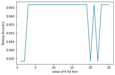
k_range = range(1, 26)
scores = {}
scores_list = []
for k in k_range:
knn = KNeighborsClassifier(n_neighbors=k)
knn.fit(x_train, y_train)
y_pred = knn.predict(x_test)
scores[k] = metrics.accuracy_score(y_test, y_pred)
scores_list.append(metrics.accuracy_score(y_test, y_pred))
%matplotlib inline
import matplotlib.pyplot as plt

plt.plot(k_range, scores_list)
plt.xlabel('value of K for Knn')
plt.ylabel('Testing Accuracy')
Text(0, 0.5, 'Testing Accuracy')
knn = KNeighborsClassifier(n_neighbors=5)
knn.fit(x,y)
KNeighborsClassifier()
classes= {0:'sentosa', 1:'versicolor', 2:'virginica'}
x_new = [[3,4,5,2],[5,4,2,2]]
y_predict = knn.predict(x_new)
print(classes[y_predict[0]])
print(classes[y_predict[1]])
versicolor
sentosa
Tugas 4 : NAIVE BAYES CLASSIFIER#
# Naive Bayes Classification

# Importing the libraries
import numpy as np
import matplotlib.pyplot as plt
import matplotlib.image as mpimg
import pandas as pd
iris=pd.read_csv("https://gist.githubusercontent.com/netj/8836201/raw/6f9306ad21398ea43cba4f7d537619d0e07d5ae3/iris.csv")
iris
| sepal.length | sepal.width | petal.length | petal.width | variety | |
|---|---|---|---|---|---|
| 0 | 5.1 | 3.5 | 1.4 | 0.2 | Setosa |
| 1 | 4.9 | 3.0 | 1.4 | 0.2 | Setosa |
| 2 | 4.7 | 3.2 | 1.3 | 0.2 | Setosa |
| 3 | 4.6 | 3.1 | 1.5 | 0.2 | Setosa |
| 4 | 5.0 | 3.6 | 1.4 | 0.2 | Setosa |
| ... | ... | ... | ... | ... | ... |
| 145 | 6.7 | 3.0 | 5.2 | 2.3 | Virginica |
| 146 | 6.3 | 2.5 | 5.0 | 1.9 | Virginica |
| 147 | 6.5 | 3.0 | 5.2 | 2.0 | Virginica |
| 148 | 6.2 | 3.4 | 5.4 | 2.3 | Virginica |
| 149 | 5.9 | 3.0 | 5.1 | 1.8 | Virginica |
150 rows × 5 columns
X = iris.iloc[:,0:4].values
y = iris.iloc[:,4].values
# Splitting the dataset into the Training set and Test set
from sklearn.model_selection import train_test_split
X_train, X_test, y_train, y_test = train_test_split(X, y, test_size = 0.20, random_state = 82)
# Feature Scaling to bring the variable in a single scale
from sklearn.preprocessing import StandardScaler
sc = StandardScaler()
X_train = sc.fit_transform(X_train)
X_test = sc.transform(X_test)
# Fitting Naive Bayes Classification to the Training set with linear kernel
from sklearn.naive_bayes import GaussianNB
nvclassifier = GaussianNB()
nvclassifier.fit(X_train, y_train)
GaussianNB()
# Predicting the Test set results
y_pred = nvclassifier.predict(X_test)
print(y_pred)
['Virginica' 'Virginica' 'Setosa' 'Setosa' 'Setosa' 'Virginica'
 'Versicolor' 'Versicolor' 'Versicolor' 'Versicolor' 'Versicolor'
 'Virginica' 'Setosa' 'Setosa' 'Setosa' 'Setosa' 'Virginica' 'Versicolor'
 'Setosa' 'Versicolor' 'Setosa' 'Virginica' 'Setosa' 'Virginica'
 'Virginica' 'Versicolor' 'Virginica' 'Setosa' 'Virginica' 'Versicolor']
#lets see the actual and predicted value side by side
y_compare = np.vstack((y_test,y_pred)).T
#actual value on the left side and predicted value on the right hand side
#printing the top 5 values
y_compare[:5,:]
array([['Virginica', 'Virginica'],
       ['Virginica', 'Virginica'],
       ['Setosa', 'Setosa'],
       ['Setosa', 'Setosa'],
       ['Setosa', 'Setosa']], dtype=object)
# Making the Confusion Matrix
from sklearn.metrics import confusion_matrix
cm = confusion_matrix(y_test, y_pred)
print(cm)
[[11  0  0]
 [ 0  8  1]
 [ 0  1  9]]
#finding accuracy from the confusion matrix.
a = cm.shape
corrPred = 0
falsePred = 0

for row in range(a[0]):
    for c in range(a[1]):
        if row == c:
            corrPred +=cm[row,c]
        else:
            falsePred += cm[row,c]
print('Correct predictions: ', corrPred)
print('False predictions', falsePred)
print ('\n\nAccuracy of the Naive Bayes Clasification is: ', corrPred/(cm.sum()))
Correct predictions:  28
False predictions 2


Accuracy of the Naive Bayes Clasification is:  0.9333333333333333
Versi 2
from sklearn.metrics import make_scorer, accuracy_score,precision_score
from sklearn.metrics import accuracy_score ,precision_score,recall_score,f1_score
from sklearn.metrics import confusion_matrix
from sklearn.model_selection import KFold,train_test_split,cross_val_score
from sklearn.naive_bayes import GaussianNB
from sklearn.model_selection import train_test_split
X = iris.iloc[:,0:4].values
y = iris.iloc[:,4].values
y.shape
(150,)
X.shape
(150, 4)
from sklearn.preprocessing import LabelEncoder
le = LabelEncoder()
y = le.fit_transform(y)
y
array([0, 0, 0, 0, 0, 0, 0, 0, 0, 0, 0, 0, 0, 0, 0, 0, 0, 0, 0, 0, 0, 0,
       0, 0, 0, 0, 0, 0, 0, 0, 0, 0, 0, 0, 0, 0, 0, 0, 0, 0, 0, 0, 0, 0,
       0, 0, 0, 0, 0, 0, 1, 1, 1, 1, 1, 1, 1, 1, 1, 1, 1, 1, 1, 1, 1, 1,
       1, 1, 1, 1, 1, 1, 1, 1, 1, 1, 1, 1, 1, 1, 1, 1, 1, 1, 1, 1, 1, 1,
       1, 1, 1, 1, 1, 1, 1, 1, 1, 1, 1, 1, 2, 2, 2, 2, 2, 2, 2, 2, 2, 2,
       2, 2, 2, 2, 2, 2, 2, 2, 2, 2, 2, 2, 2, 2, 2, 2, 2, 2, 2, 2, 2, 2,
       2, 2, 2, 2, 2, 2, 2, 2, 2, 2, 2, 2, 2, 2, 2, 2, 2, 2])
#Train and Test split
X_train,X_test,y_train,y_test=train_test_split(X,y,test_size=0.3,random_state=0)
gaussian = GaussianNB()
gaussian.fit(X_train, y_train)
Y_pred = gaussian.predict(X_test)
accuracy_nb=round(accuracy_score(y_test,Y_pred)* 100, 2)
acc_gaussian = round(gaussian.score(X_train, y_train) * 100, 2)

cm = confusion_matrix(y_test, Y_pred)
accuracy = accuracy_score(y_test,Y_pred)
precision =precision_score(y_test, Y_pred,average='micro')
recall =  recall_score(y_test, Y_pred,average='micro')
f1 = f1_score(y_test,Y_pred,average='micro')
print('Confusion matrix for Naive Bayes\n',cm)
print('accuracy_Naive Bayes: %.3f' %accuracy)
print('precision_Naive Bayes: %.3f' %precision)
print('recall_Naive Bayes: %.3f' %recall)
print('f1-score_Naive Bayes : %.3f' %f1)
Confusion matrix for Naive Bayes
 [[16  0  0]
 [ 0 18  0]
 [ 0  0 11]]
accuracy_Naive Bayes: 1.000
precision_Naive Bayes: 1.000
recall_Naive Bayes: 1.000
f1-score_Naive Bayes : 1.000
from sklearn.svm import SVC
from sklearn.ensemble import BaggingClassifier
from sklearn.datasets import make_classification
X, y = make_classification(n_samples=100, n_features=4,
                              n_informative=2, n_redundant=0,
                              random_state=0, shuffle=False)
clf = BaggingClassifier(base_estimator=SVC(),
                         n_estimators=10, random_state=0).fit(X, y)
clf.predict([[0, 0, 0, 0]])
array([1])
Versi Bagging
import pandas as pd
import numpy as np
import matplotlib.pyplot as plt
N = 1000
data = np.arange(N)
BS = np.random.choice(data, size = N)
BS_unique = set(BS)
len(BS_unique)
630
wine_pd = pd.read_csv("https://raw.githubusercontent.com/Rosita19/datamining/main/wine.csv")
wine_pd.head()
| Alcohol | Malic_acid | Ash | Alcalinity_of_ash | Magnesium | Total_phenols | Flavanoids | Nonflavanoid_phenols | Proanthocyanins | Color_intensity | Hue | OD280/OD315_of_diluted_wines | Proline | class | |
|---|---|---|---|---|---|---|---|---|---|---|---|---|---|---|
| 0 | 14.23 | 1.71 | 2.43 | 15.6 | 127 | 2.80 | 3.06 | 0.28 | 2.29 | 5.64 | 1.04 | 3.92 | 1065 | Type1 |
| 1 | 13.20 | 1.78 | 2.14 | 11.2 | 100 | 2.65 | 2.76 | 0.26 | 1.28 | 4.38 | 1.05 | 3.40 | 1050 | Type1 |
| 2 | 13.16 | 2.36 | 2.67 | 18.6 | 101 | 2.80 | 3.24 | 0.30 | 2.81 | 5.68 | 1.03 | 3.17 | 1185 | Type1 |
| 3 | 14.37 | 1.95 | 2.50 | 16.8 | 113 | 3.85 | 3.49 | 0.24 | 2.18 | 7.80 | 0.86 | 3.45 | 1480 | Type1 |
| 4 | 13.24 | 2.59 | 2.87 | 21.0 | 118 | 2.80 | 2.69 | 0.39 | 1.82 | 4.32 | 1.04 | 2.93 | 735 | Type1 |
y = wine_pd.pop('class').values
X = wine_pd.values
X.shape
(178, 13)
from sklearn.neighbors import KNeighborsClassifier
from sklearn.tree import DecisionTreeClassifier
from sklearn.neural_network import MLPClassifier
from sklearn.naive_bayes import GaussianNB
from sklearn.linear_model import LogisticRegression
from sklearn.model_selection import cross_val_score, cross_validate, RepeatedKFold
from sklearn.model_selection import train_test_split
from sklearn.ensemble import BaggingClassifier
from sklearn.preprocessing import StandardScaler
from sklearn.pipeline import Pipeline
dtree = DecisionTreeClassifier(criterion='entropy')
# A helper function that will run RepeatedKFold cross validation for a range
# of ensemble sizes (est_range).
# Takes, the estimator, n_reps and the range as arguments.
def eval_bag_est_range(the_est, n_reps, est_range, folds = 10):
    n_est_dict = {}
    for n_est in est_range:
        the_bag = BaggingClassifier(the_est,
                            n_estimators = n_est,
                            max_samples = 1.0, # bootstrap resampling
                            bootstrap = True)
        bag_cv = cross_validate(the_bag, X, y, n_jobs=-1,
                                cv=RepeatedKFold(n_splits=folds, n_repeats=n_reps))
        n_est_dict[n_est]=bag_cv['test_score'].mean()
    return n_est_dict
kNNpipe  = Pipeline(steps=[ ('scaler', StandardScaler()),
                           ('classifier', KNeighborsClassifier(n_neighbors=1))])

NNPipe = Pipeline(steps=[ ('scaler', StandardScaler()),
                           ('classifier', MLPClassifier(solver='lbfgs', alpha=1e-5,
                                                        hidden_layer_sizes=(5, 2)))])
res_kNN_bag = eval_bag_est_range(kNNpipe, 10, range(2,16))
kNN_list = sorted(res_kNN_bag.items()) # sorted by key, return a list of tuples
nc, kNN_accs = zip(*kNN_list) # unpack a list of pairs into two tuples
NN_list = sorted(res_NN_bag.items()) # sorted by key, return a list of tuples
nc, NN_accs = zip(*NN_list) # unpack a list of pairs into two tuples

f = plt.figure(figsize=(5,4))

plt.plot(nc, NN_accs, lw = 2, color = 'r', label = 'Neural Net')
plt.plot(nc, kNN_accs, lw = 2, color = 'orange', label = 'k-NN')

plt.xlabel("Number of estimators")
plt.ylabel("Accuracy")
plt.ylim([0.94,1])
plt.legend(loc = 'upper left')
plt.grid(axis = 'y')
f.savefig('bag-est-plot.pdf')
---------------------------------------------------------------------------
NameError                                 Traceback (most recent call last)
<ipython-input-53-6900fa04807b> in <module>
      1 kNN_list = sorted(res_kNN_bag.items()) # sorted by key, return a list of tuples
      2 nc, kNN_accs = zip(*kNN_list) # unpack a list of pairs into two tuples
----> 3 NN_list = sorted(res_NN_bag.items()) # sorted by key, return a list of tuples
      4 nc, NN_accs = zip(*NN_list) # unpack a list of pairs into two tuples
      5

NameError: name 'res_NN_bag' is not defined
Tugas 5 : K-Means Clustering#
Import Library
import pandas as pd
import numpy as np
import matplotlib.pyplot as plt
import seaborn as sns
from sklearn.cluster import KMeans
from sklearn.metrics import silhouette_score
from sklearn.preprocessing import MinMaxScaler
Import Data Dari Github
from os import X_OK
iris = pd.read_csv("https://raw.githubusercontent.com/Rosita19/datamining/main/iris.csv")
X_OK = iris.iloc[:, [0, 1, 2, 3]].values
Menampilkan Data Iris tanpa label
X = iris.values[:, 0:4]
y = iris.values[:, 4]
X
array([[5.1, 3.5, 1.4, 0.2],
       [4.9, 3.0, 1.4, 0.2],
       [4.7, 3.2, 1.3, 0.2],
       [4.6, 3.1, 1.5, 0.2],
       [5.0, 3.6, 1.4, 0.2],
       [5.4, 3.9, 1.7, 0.4],
       [4.6, 3.4, 1.4, 0.3],
       [5.0, 3.4, 1.5, 0.2],
       [4.4, 2.9, 1.4, 0.2],
       [4.9, 3.1, 1.5, 0.1],
       [5.4, 3.7, 1.5, 0.2],
       [4.8, 3.4, 1.6, 0.2],
       [4.8, 3.0, 1.4, 0.1],
       [4.3, 3.0, 1.1, 0.1],
       [5.8, 4.0, 1.2, 0.2],
       [5.7, 4.4, 1.5, 0.4],
       [5.4, 3.9, 1.3, 0.4],
       [5.1, 3.5, 1.4, 0.3],
       [5.7, 3.8, 1.7, 0.3],
       [5.1, 3.8, 1.5, 0.3],
       [5.4, 3.4, 1.7, 0.2],
       [5.1, 3.7, 1.5, 0.4],
       [4.6, 3.6, 1.0, 0.2],
       [5.1, 3.3, 1.7, 0.5],
       [4.8, 3.4, 1.9, 0.2],
       [5.0, 3.0, 1.6, 0.2],
       [5.0, 3.4, 1.6, 0.4],
       [5.2, 3.5, 1.5, 0.2],
       [5.2, 3.4, 1.4, 0.2],
       [4.7, 3.2, 1.6, 0.2],
       [4.8, 3.1, 1.6, 0.2],
       [5.4, 3.4, 1.5, 0.4],
       [5.2, 4.1, 1.5, 0.1],
       [5.5, 4.2, 1.4, 0.2],
       [4.9, 3.1, 1.5, 0.1],
       [5.0, 3.2, 1.2, 0.2],
       [5.5, 3.5, 1.3, 0.2],
       [4.9, 3.1, 1.5, 0.1],
       [4.4, 3.0, 1.3, 0.2],
       [5.1, 3.4, 1.5, 0.2],
       [5.0, 3.5, 1.3, 0.3],
       [4.5, 2.3, 1.3, 0.3],
       [4.4, 3.2, 1.3, 0.2],
       [5.0, 3.5, 1.6, 0.6],
       [5.1, 3.8, 1.9, 0.4],
       [4.8, 3.0, 1.4, 0.3],
       [5.1, 3.8, 1.6, 0.2],
       [4.6, 3.2, 1.4, 0.2],
       [5.3, 3.7, 1.5, 0.2],
       [5.0, 3.3, 1.4, 0.2],
       [7.0, 3.2, 4.7, 1.4],
       [6.4, 3.2, 4.5, 1.5],
       [6.9, 3.1, 4.9, 1.5],
       [5.5, 2.3, 4.0, 1.3],
       [6.5, 2.8, 4.6, 1.5],
       [5.7, 2.8, 4.5, 1.3],
       [6.3, 3.3, 4.7, 1.6],
       [4.9, 2.4, 3.3, 1.0],
       [6.6, 2.9, 4.6, 1.3],
       [5.2, 2.7, 3.9, 1.4],
       [5.0, 2.0, 3.5, 1.0],
       [5.9, 3.0, 4.2, 1.5],
       [6.0, 2.2, 4.0, 1.0],
       [6.1, 2.9, 4.7, 1.4],
       [5.6, 2.9, 3.6, 1.3],
       [6.7, 3.1, 4.4, 1.4],
       [5.6, 3.0, 4.5, 1.5],
       [5.8, 2.7, 4.1, 1.0],
       [6.2, 2.2, 4.5, 1.5],
       [5.6, 2.5, 3.9, 1.1],
       [5.9, 3.2, 4.8, 1.8],
       [6.1, 2.8, 4.0, 1.3],
       [6.3, 2.5, 4.9, 1.5],
       [6.1, 2.8, 4.7, 1.2],
       [6.4, 2.9, 4.3, 1.3],
       [6.6, 3.0, 4.4, 1.4],
       [6.8, 2.8, 4.8, 1.4],
       [6.7, 3.0, 5.0, 1.7],
       [6.0, 2.9, 4.5, 1.5],
       [5.7, 2.6, 3.5, 1.0],
       [5.5, 2.4, 3.8, 1.1],
       [5.5, 2.4, 3.7, 1.0],
       [5.8, 2.7, 3.9, 1.2],
       [6.0, 2.7, 5.1, 1.6],
       [5.4, 3.0, 4.5, 1.5],
       [6.0, 3.4, 4.5, 1.6],
       [6.7, 3.1, 4.7, 1.5],
       [6.3, 2.3, 4.4, 1.3],
       [5.6, 3.0, 4.1, 1.3],
       [5.5, 2.5, 4.0, 1.3],
       [5.5, 2.6, 4.4, 1.2],
       [6.1, 3.0, 4.6, 1.4],
       [5.8, 2.6, 4.0, 1.2],
       [5.0, 2.3, 3.3, 1.0],
       [5.6, 2.7, 4.2, 1.3],
       [5.7, 3.0, 4.2, 1.2],
       [5.7, 2.9, 4.2, 1.3],
       [6.2, 2.9, 4.3, 1.3],
       [5.1, 2.5, 3.0, 1.1],
       [5.7, 2.8, 4.1, 1.3],
       [6.3, 3.3, 6.0, 2.5],
       [5.8, 2.7, 5.1, 1.9],
       [7.1, 3.0, 5.9, 2.1],
       [6.3, 2.9, 5.6, 1.8],
       [6.5, 3.0, 5.8, 2.2],
       [7.6, 3.0, 6.6, 2.1],
       [4.9, 2.5, 4.5, 1.7],
       [7.3, 2.9, 6.3, 1.8],
       [6.7, 2.5, 5.8, 1.8],
       [7.2, 3.6, 6.1, 2.5],
       [6.5, 3.2, 5.1, 2.0],
       [6.4, 2.7, 5.3, 1.9],
       [6.8, 3.0, 5.5, 2.1],
       [5.7, 2.5, 5.0, 2.0],
       [5.8, 2.8, 5.1, 2.4],
       [6.4, 3.2, 5.3, 2.3],
       [6.5, 3.0, 5.5, 1.8],
       [7.7, 3.8, 6.7, 2.2],
       [7.7, 2.6, 6.9, 2.3],
       [6.0, 2.2, 5.0, 1.5],
       [6.9, 3.2, 5.7, 2.3],
       [5.6, 2.8, 4.9, 2.0],
       [7.7, 2.8, 6.7, 2.0],
       [6.3, 2.7, 4.9, 1.8],
       [6.7, 3.3, 5.7, 2.1],
       [7.2, 3.2, 6.0, 1.8],
       [6.2, 2.8, 4.8, 1.8],
       [6.1, 3.0, 4.9, 1.8],
       [6.4, 2.8, 5.6, 2.1],
       [7.2, 3.0, 5.8, 1.6],
       [7.4, 2.8, 6.1, 1.9],
       [7.9, 3.8, 6.4, 2.0],
       [6.4, 2.8, 5.6, 2.2],
       [6.3, 2.8, 5.1, 1.5],
       [6.1, 2.6, 5.6, 1.4],
       [7.7, 3.0, 6.1, 2.3],
       [6.3, 3.4, 5.6, 2.4],
       [6.4, 3.1, 5.5, 1.8],
       [6.0, 3.0, 4.8, 1.8],
       [6.9, 3.1, 5.4, 2.1],
       [6.7, 3.1, 5.6, 2.4],
       [6.9, 3.1, 5.1, 2.3],
       [5.8, 2.7, 5.1, 1.9],
       [6.8, 3.2, 5.9, 2.3],
       [6.7, 3.3, 5.7, 2.5],
       [6.7, 3.0, 5.2, 2.3],
       [6.3, 2.5, 5.0, 1.9],
       [6.5, 3.0, 5.2, 2.0],
       [6.2, 3.4, 5.4, 2.3],
       [5.9, 3.0, 5.1, 1.8]], dtype=object)
iris.info()
iris[0:10]
<class 'pandas.core.frame.DataFrame'>
RangeIndex: 150 entries, 0 to 149
Data columns (total 5 columns):
 #   Column        Non-Null Count  Dtype
---  ------        --------------  -----
 0   sepal_length  150 non-null    float64
 1   sepal_width   150 non-null    float64
 2   petal_length  150 non-null    float64
 3   petal_width   150 non-null    float64
 4   species       150 non-null    object
dtypes: float64(4), object(1)
memory usage: 6.0+ KB
| sepal_length | sepal_width | petal_length | petal_width | species | |
|---|---|---|---|---|---|
| 0 | 5.1 | 3.5 | 1.4 | 0.2 | setosa |
| 1 | 4.9 | 3.0 | 1.4 | 0.2 | setosa |
| 2 | 4.7 | 3.2 | 1.3 | 0.2 | setosa |
| 3 | 4.6 | 3.1 | 1.5 | 0.2 | setosa |
| 4 | 5.0 | 3.6 | 1.4 | 0.2 | setosa |
| 5 | 5.4 | 3.9 | 1.7 | 0.4 | setosa |
| 6 | 4.6 | 3.4 | 1.4 | 0.3 | setosa |
| 7 | 5.0 | 3.4 | 1.5 | 0.2 | setosa |
| 8 | 4.4 | 2.9 | 1.4 | 0.2 | setosa |
| 9 | 4.9 | 3.1 | 1.5 | 0.1 | setosa |
#Frequency distribution of species"
iris_outcome = pd.crosstab(index=iris["species"],  # Make a crosstab
columns="count")      # Name the count column

iris_outcome
| col_0 | count |
|---|---|
| species | |
| setosa | 50 |
| versicolor | 50 |
| virginica | 50 |
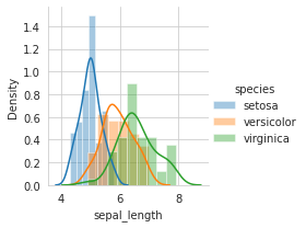
iris_setosa=iris.loc[iris["species"]=="Iris-setosa"]
iris_virginica=iris.loc[iris["species"]=="Iris-virginica"]
iris_versicolor=iris.loc[iris["species"]=="Iris-versicolor"]
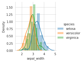
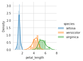
sns.FacetGrid(iris,hue="species",size=3).map(sns.distplot,"sepal_length").add_legend()
sns.FacetGrid(iris,hue="species",size=3).map(sns.distplot,"sepal_width").add_legend()
sns.FacetGrid(iris,hue="species",size=3).map(sns.distplot,"petal_length").add_legend()
plt.show()
/usr/local/lib/python3.7/dist-packages/seaborn/axisgrid.py:337: UserWarning: The `size` parameter has been renamed to `height`; please update your code.
  warnings.warn(msg, UserWarning)
/usr/local/lib/python3.7/dist-packages/seaborn/distributions.py:2619: FutureWarning: `distplot` is a deprecated function and will be removed in a future version. Please adapt your code to use either `displot` (a figure-level function with similar flexibility) or `histplot` (an axes-level function for histograms).
  warnings.warn(msg, FutureWarning)
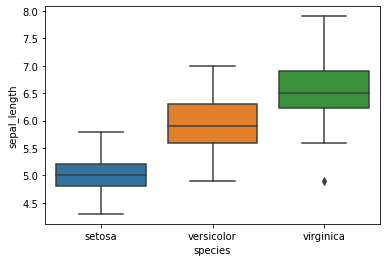
sns.boxplot(x="species",y="sepal_length",data=iris)
plt.show()
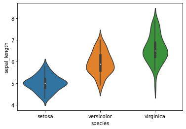
sns.violinplot(x="species",y="sepal_length",data=iris)
plt.show()
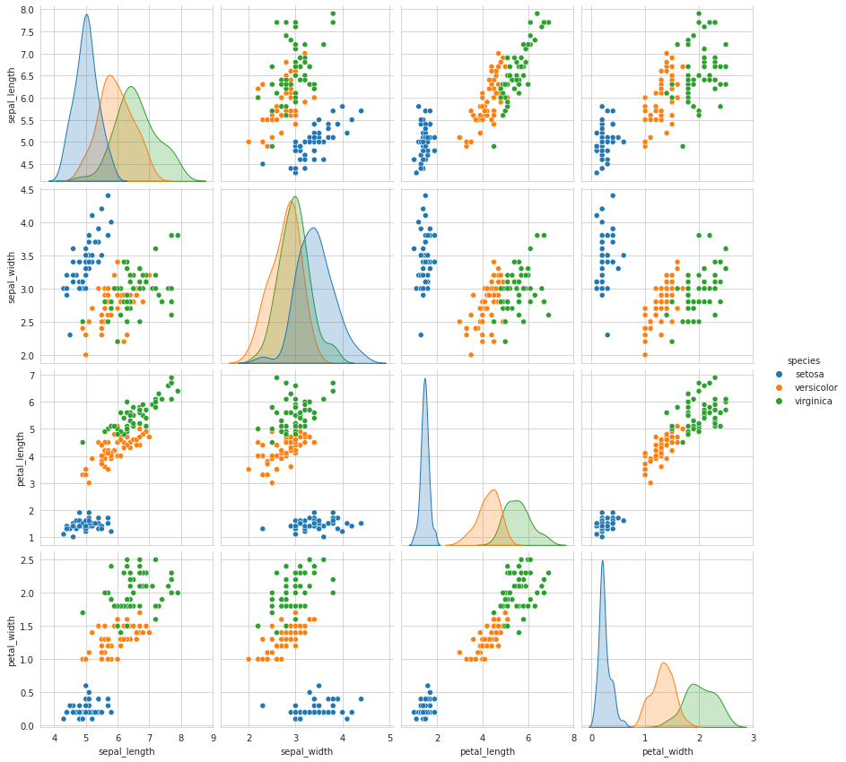
sns.set_style("whitegrid")
sns.pairplot(iris,hue="species",size=3);
plt.show()
/usr/local/lib/python3.7/dist-packages/seaborn/axisgrid.py:2076: UserWarning: The `size` parameter has been renamed to `height`; please update your code.
  warnings.warn(msg, UserWarning)
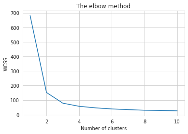
#Finding the optimum number of clusters for k-means classification
from sklearn.cluster import KMeans
wcss = []

for i in range(1, 11):
    kmeans = KMeans(n_clusters = i, init = 'k-means++', max_iter = 300, n_init = 10, random_state = 0)
    kmeans.fit(x)
    wcss.append(kmeans.inertia_)
wcss
[681.3706,
 152.3479517603579,
 78.851441426146,
 57.22847321428572,
 46.47223015873017,
 39.03998724608726,
 34.29971212121213,
 30.06311061745273,
 28.271721728563833,
 26.09432474054042]
plt.plot(range(1, 11), wcss)
plt.title('The elbow method')
plt.xlabel('Number of clusters')
plt.ylabel('WCSS') #within cluster sum of squares
plt.show()
kmeans = KMeans(n_clusters = 3, init = 'k-means++', max_iter = 300, n_init = 10, random_state = 0)
y_kmeans = kmeans.fit_predict(x)
y_kmeans
array([1, 1, 1, 1, 1, 1, 1, 1, 1, 1, 1, 1, 1, 1, 1, 1, 1, 1, 1, 1, 1, 1,
       1, 1, 1, 1, 1, 1, 1, 1, 1, 1, 1, 1, 1, 1, 1, 1, 1, 1, 1, 1, 1, 1,
       1, 1, 1, 1, 1, 1, 0, 0, 2, 0, 0, 0, 0, 0, 0, 0, 0, 0, 0, 0, 0, 0,
       0, 0, 0, 0, 0, 0, 0, 0, 0, 0, 0, 2, 0, 0, 0, 0, 0, 0, 0, 0, 0, 0,
       0, 0, 0, 0, 0, 0, 0, 0, 0, 0, 0, 0, 2, 0, 2, 2, 2, 2, 0, 2, 2, 2,
       2, 2, 2, 0, 0, 2, 2, 2, 2, 0, 2, 0, 2, 0, 2, 2, 0, 0, 2, 2, 2, 2,
       2, 0, 2, 2, 2, 2, 0, 2, 2, 2, 0, 2, 2, 2, 0, 2, 2, 0], dtype=int32)
from  sklearn.decomposition import PCA
pca=PCA(n_components=2)
X_new=pca.fit_transform(x)
X_new
array([[-2.68412563,  0.31939725],
       [-2.71414169, -0.17700123],
       [-2.88899057, -0.14494943],
       [-2.74534286, -0.31829898],
       [-2.72871654,  0.32675451],
       [-2.28085963,  0.74133045],
       [-2.82053775, -0.08946138],
       [-2.62614497,  0.16338496],
       [-2.88638273, -0.57831175],
       [-2.6727558 , -0.11377425],
       [-2.50694709,  0.6450689 ],
       [-2.61275523,  0.01472994],
       [-2.78610927, -0.235112  ],
       [-3.22380374, -0.51139459],
       [-2.64475039,  1.17876464],
       [-2.38603903,  1.33806233],
       [-2.62352788,  0.81067951],
       [-2.64829671,  0.31184914],
       [-2.19982032,  0.87283904],
       [-2.5879864 ,  0.51356031],
       [-2.31025622,  0.39134594],
       [-2.54370523,  0.43299606],
       [-3.21593942,  0.13346807],
       [-2.30273318,  0.09870885],
       [-2.35575405, -0.03728186],
       [-2.50666891, -0.14601688],
       [-2.46882007,  0.13095149],
       [-2.56231991,  0.36771886],
       [-2.63953472,  0.31203998],
       [-2.63198939, -0.19696122],
       [-2.58739848, -0.20431849],
       [-2.4099325 ,  0.41092426],
       [-2.64886233,  0.81336382],
       [-2.59873675,  1.09314576],
       [-2.63692688, -0.12132235],
       [-2.86624165,  0.06936447],
       [-2.62523805,  0.59937002],
       [-2.80068412,  0.26864374],
       [-2.98050204, -0.48795834],
       [-2.59000631,  0.22904384],
       [-2.77010243,  0.26352753],
       [-2.84936871, -0.94096057],
       [-2.99740655, -0.34192606],
       [-2.40561449,  0.18887143],
       [-2.20948924,  0.43666314],
       [-2.71445143, -0.2502082 ],
       [-2.53814826,  0.50377114],
       [-2.83946217, -0.22794557],
       [-2.54308575,  0.57941002],
       [-2.70335978,  0.10770608],
       [ 1.28482569,  0.68516047],
       [ 0.93248853,  0.31833364],
       [ 1.46430232,  0.50426282],
       [ 0.18331772, -0.82795901],
       [ 1.08810326,  0.07459068],
       [ 0.64166908, -0.41824687],
       [ 1.09506066,  0.28346827],
       [-0.74912267, -1.00489096],
       [ 1.04413183,  0.2283619 ],
       [-0.0087454 , -0.72308191],
       [-0.50784088, -1.26597119],
       [ 0.51169856, -0.10398124],
       [ 0.26497651, -0.55003646],
       [ 0.98493451, -0.12481785],
       [-0.17392537, -0.25485421],
       [ 0.92786078,  0.46717949],
       [ 0.66028376, -0.35296967],
       [ 0.23610499, -0.33361077],
       [ 0.94473373, -0.54314555],
       [ 0.04522698, -0.58383438],
       [ 1.11628318, -0.08461685],
       [ 0.35788842, -0.06892503],
       [ 1.29818388, -0.32778731],
       [ 0.92172892, -0.18273779],
       [ 0.71485333,  0.14905594],
       [ 0.90017437,  0.32850447],
       [ 1.33202444,  0.24444088],
       [ 1.55780216,  0.26749545],
       [ 0.81329065, -0.1633503 ],
       [-0.30558378, -0.36826219],
       [-0.06812649, -0.70517213],
       [-0.18962247, -0.68028676],
       [ 0.13642871, -0.31403244],
       [ 1.38002644, -0.42095429],
       [ 0.58800644, -0.48428742],
       [ 0.80685831,  0.19418231],
       [ 1.22069088,  0.40761959],
       [ 0.81509524, -0.37203706],
       [ 0.24595768, -0.2685244 ],
       [ 0.16641322, -0.68192672],
       [ 0.46480029, -0.67071154],
       [ 0.8908152 , -0.03446444],
       [ 0.23054802, -0.40438585],
       [-0.70453176, -1.01224823],
       [ 0.35698149, -0.50491009],
       [ 0.33193448, -0.21265468],
       [ 0.37621565, -0.29321893],
       [ 0.64257601,  0.01773819],
       [-0.90646986, -0.75609337],
       [ 0.29900084, -0.34889781],
       [ 2.53119273, -0.00984911],
       [ 1.41523588, -0.57491635],
       [ 2.61667602,  0.34390315],
       [ 1.97153105, -0.1797279 ],
       [ 2.35000592, -0.04026095],
       [ 3.39703874,  0.55083667],
       [ 0.52123224, -1.19275873],
       [ 2.93258707,  0.3555    ],
       [ 2.32122882, -0.2438315 ],
       [ 2.91675097,  0.78279195],
       [ 1.66177415,  0.24222841],
       [ 1.80340195, -0.21563762],
       [ 2.1655918 ,  0.21627559],
       [ 1.34616358, -0.77681835],
       [ 1.58592822, -0.53964071],
       [ 1.90445637,  0.11925069],
       [ 1.94968906,  0.04194326],
       [ 3.48705536,  1.17573933],
       [ 3.79564542,  0.25732297],
       [ 1.30079171, -0.76114964],
       [ 2.42781791,  0.37819601],
       [ 1.19900111, -0.60609153],
       [ 3.49992004,  0.4606741 ],
       [ 1.38876613, -0.20439933],
       [ 2.2754305 ,  0.33499061],
       [ 2.61409047,  0.56090136],
       [ 1.25850816, -0.17970479],
       [ 1.29113206, -0.11666865],
       [ 2.12360872, -0.20972948],
       [ 2.38800302,  0.4646398 ],
       [ 2.84167278,  0.37526917],
       [ 3.23067366,  1.37416509],
       [ 2.15943764, -0.21727758],
       [ 1.44416124, -0.14341341],
       [ 1.78129481, -0.49990168],
       [ 3.07649993,  0.68808568],
       [ 2.14424331,  0.1400642 ],
       [ 1.90509815,  0.04930053],
       [ 1.16932634, -0.16499026],
       [ 2.10761114,  0.37228787],
       [ 2.31415471,  0.18365128],
       [ 1.9222678 ,  0.40920347],
       [ 1.41523588, -0.57491635],
       [ 2.56301338,  0.2778626 ],
       [ 2.41874618,  0.3047982 ],
       [ 1.94410979,  0.1875323 ],
       [ 1.52716661, -0.37531698],
       [ 1.76434572,  0.07885885],
       [ 1.90094161,  0.11662796],
       [ 1.39018886, -0.28266094]])
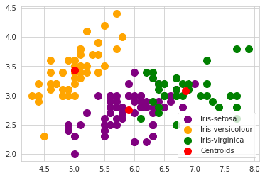
#Visualising the clusters
plt.scatter(x[y_kmeans == 0, 0], x[y_kmeans == 0, 1], s = 100, c = 'purple', label = 'Iris-setosa')
plt.scatter(x[y_kmeans == 1, 0], x[y_kmeans == 1, 1], s = 100, c = 'orange', label = 'Iris-versicolour')
plt.scatter(x[y_kmeans == 2, 0], x[y_kmeans == 2, 1], s = 100, c = 'green', label = 'Iris-virginica')

#Plotting the centroids of the clusters
plt.scatter(kmeans.cluster_centers_[:, 0], kmeans.cluster_centers_[:,1], s = 100, c = 'red', label = 'Centroids')

plt.legend()
<matplotlib.legend.Legend at 0x7f6cfc1dde10>
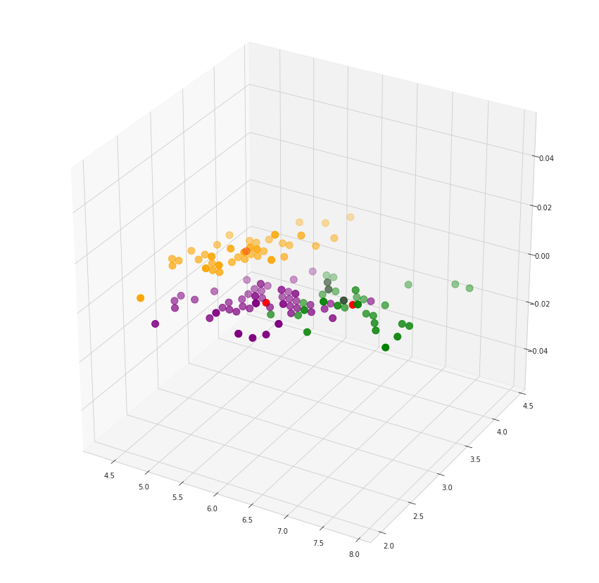
# 3d scatterplot using matplotlib

fig = plt.figure(figsize = (15,15))
ax = fig.add_subplot(111, projection='3d')
plt.scatter(x[y_kmeans == 0, 0], x[y_kmeans == 0, 1], s = 100, c = 'purple', label = 'Iris-setosa')
plt.scatter(x[y_kmeans == 1, 0], x[y_kmeans == 1, 1], s = 100, c = 'orange', label = 'Iris-versicolour')
plt.scatter(x[y_kmeans == 2, 0], x[y_kmeans == 2, 1], s = 100, c = 'green', label = 'Iris-virginica')

#Plotting the centroids of the clusters
plt.scatter(kmeans.cluster_centers_[:, 0], kmeans.cluster_centers_[:,1], s = 100, c = 'red', label = 'Centroids')
plt.show()
Tugas 6 : Decision Tree (Pohon Keputusan)#
from sklearn import tree
import graphviz
from sklearn.tree import DecisionTreeClassifier
from sklearn.model_selection import train_test_split, cross_val_score
iris = pd.read_csv("https://raw.githubusercontent.com/Rosita19/datamining/main/iris.csv")
iris
| sepal_length | sepal_width | petal_length | petal_width | species | |
|---|---|---|---|---|---|
| 0 | 5.1 | 3.5 | 1.4 | 0.2 | setosa |
| 1 | 4.9 | 3.0 | 1.4 | 0.2 | setosa |
| 2 | 4.7 | 3.2 | 1.3 | 0.2 | setosa |
| 3 | 4.6 | 3.1 | 1.5 | 0.2 | setosa |
| 4 | 5.0 | 3.6 | 1.4 | 0.2 | setosa |
| ... | ... | ... | ... | ... | ... |
| 145 | 6.7 | 3.0 | 5.2 | 2.3 | virginica |
| 146 | 6.3 | 2.5 | 5.0 | 1.9 | virginica |
| 147 | 6.5 | 3.0 | 5.2 | 2.0 | virginica |
| 148 | 6.2 | 3.4 | 5.4 | 2.3 | virginica |
| 149 | 5.9 | 3.0 | 5.1 | 1.8 | virginica |
150 rows × 5 columns
from sklearn import tree
X = [[0, 0], [1, 1]]
Y = [0, 1]
clf = tree.DecisionTreeClassifier()
clf = clf.fit(X, Y)
clf.predict([[2., 2.]])
array([1])
clf.predict_proba([[2., 2.]])
array([[0., 1.]])
from sklearn.datasets import load_iris
from sklearn import tree
iris = load_iris()
X, y = iris.data, iris.target
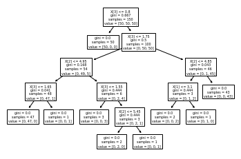
clf = tree.DecisionTreeClassifier()
clf = clf.fit(X, y)
tree.plot_tree(clf)
[Text(0.5, 0.9166666666666666, 'X[3] <= 0.8\ngini = 0.667\nsamples = 150\nvalue = [50, 50, 50]'),
 Text(0.4230769230769231, 0.75, 'gini = 0.0\nsamples = 50\nvalue = [50, 0, 0]'),
 Text(0.5769230769230769, 0.75, 'X[3] <= 1.75\ngini = 0.5\nsamples = 100\nvalue = [0, 50, 50]'),
 Text(0.3076923076923077, 0.5833333333333334, 'X[2] <= 4.95\ngini = 0.168\nsamples = 54\nvalue = [0, 49, 5]'),
 Text(0.15384615384615385, 0.4166666666666667, 'X[3] <= 1.65\ngini = 0.041\nsamples = 48\nvalue = [0, 47, 1]'),
 Text(0.07692307692307693, 0.25, 'gini = 0.0\nsamples = 47\nvalue = [0, 47, 0]'),
 Text(0.23076923076923078, 0.25, 'gini = 0.0\nsamples = 1\nvalue = [0, 0, 1]'),
 Text(0.46153846153846156, 0.4166666666666667, 'X[3] <= 1.55\ngini = 0.444\nsamples = 6\nvalue = [0, 2, 4]'),
 Text(0.38461538461538464, 0.25, 'gini = 0.0\nsamples = 3\nvalue = [0, 0, 3]'),
 Text(0.5384615384615384, 0.25, 'X[2] <= 5.45\ngini = 0.444\nsamples = 3\nvalue = [0, 2, 1]'),
 Text(0.46153846153846156, 0.08333333333333333, 'gini = 0.0\nsamples = 2\nvalue = [0, 2, 0]'),
 Text(0.6153846153846154, 0.08333333333333333, 'gini = 0.0\nsamples = 1\nvalue = [0, 0, 1]'),
 Text(0.8461538461538461, 0.5833333333333334, 'X[2] <= 4.85\ngini = 0.043\nsamples = 46\nvalue = [0, 1, 45]'),
 Text(0.7692307692307693, 0.4166666666666667, 'X[1] <= 3.1\ngini = 0.444\nsamples = 3\nvalue = [0, 1, 2]'),
 Text(0.6923076923076923, 0.25, 'gini = 0.0\nsamples = 2\nvalue = [0, 0, 2]'),
 Text(0.8461538461538461, 0.25, 'gini = 0.0\nsamples = 1\nvalue = [0, 1, 0]'),
 Text(0.9230769230769231, 0.4166666666666667, 'gini = 0.0\nsamples = 43\nvalue = [0, 0, 43]')]
import graphviz
dot_data = tree.export_graphviz(clf, out_file=None)
graph = graphviz.Source(dot_data)
graph.render("iris")
'iris.pdf'
dot_data = tree.export_graphviz(clf, out_file=None,
                      feature_names=iris.feature_names,
                      class_names=iris.target_names,
                      filled=True, rounded=True,
                      special_characters=True)
graph = graphviz.Source(dot_data)
graph

from sklearn.datasets import load_iris
from sklearn.tree import DecisionTreeClassifier
from sklearn.tree import export_text
iris = load_iris()
decision_tree = DecisionTreeClassifier(random_state=0, max_depth=2)
decision_tree = decision_tree.fit(iris.data, iris.target)
r = export_text(decision_tree, feature_names=iris['feature_names'])
print(r)
|--- petal width (cm) <= 0.80
|   |--- class: 0
|--- petal width (cm) >  0.80
|   |--- petal width (cm) <= 1.75
|   |   |--- class: 1
|   |--- petal width (cm) >  1.75
|   |   |--- class: 2
UTS#
Lakukan analisa terhadap data pada https://archive.ics.uci.edu/ml/datasets/Breast+Cancer+Coimbra dengan menggunakan klasifikasi
metode Naive Bayes Classifier
metode pohon keputusan (Desision Tree)
1. Metode Naive Bayes Classifier#
# Naive Bayes Classification

# Importing the libraries
import numpy as np
import matplotlib.pyplot as plt
import matplotlib.image as mpimg
import pandas as pd
dataR2="https://raw.githubusercontent.com/Rosita19/datamining/main/dataR2.csv"
data = pd.read_csv(dataR2)
data
| Age | BMI | Glucose | Insulin | HOMA | Leptin | Adiponectin | Resistin | MCP.1 | Classification | |
|---|---|---|---|---|---|---|---|---|---|---|
| 0 | 48 | 23.500000 | 70 | 2.707 | 0.467409 | 8.8071 | 9.702400 | 7.99585 | 417.114 | 1 |
| 1 | 83 | 20.690495 | 92 | 3.115 | 0.706897 | 8.8438 | 5.429285 | 4.06405 | 468.786 | 1 |
| 2 | 82 | 23.124670 | 91 | 4.498 | 1.009651 | 17.9393 | 22.432040 | 9.27715 | 554.697 | 1 |
| 3 | 68 | 21.367521 | 77 | 3.226 | 0.612725 | 9.8827 | 7.169560 | 12.76600 | 928.220 | 1 |
| 4 | 86 | 21.111111 | 92 | 3.549 | 0.805386 | 6.6994 | 4.819240 | 10.57635 | 773.920 | 1 |
| ... | ... | ... | ... | ... | ... | ... | ... | ... | ... | ... |
| 111 | 45 | 26.850000 | 92 | 3.330 | 0.755688 | 54.6800 | 12.100000 | 10.96000 | 268.230 | 2 |
| 112 | 62 | 26.840000 | 100 | 4.530 | 1.117400 | 12.4500 | 21.420000 | 7.32000 | 330.160 | 2 |
| 113 | 65 | 32.050000 | 97 | 5.730 | 1.370998 | 61.4800 | 22.540000 | 10.33000 | 314.050 | 2 |
| 114 | 72 | 25.590000 | 82 | 2.820 | 0.570392 | 24.9600 | 33.750000 | 3.27000 | 392.460 | 2 |
| 115 | 86 | 27.180000 | 138 | 19.910 | 6.777364 | 90.2800 | 14.110000 | 4.35000 | 90.090 | 2 |
116 rows × 10 columns
data.shape
(116, 10)
#Pilih data menjadi variabel independen 'X' dan variabel 'y'
X = data.iloc[:,:9].values
y = data['Classification'].values
# Memisahkan datauts ke dalam set Pelatihan dan set Testing
from sklearn.model_selection import train_test_split
X_train, X_test, y_train, y_test = train_test_split(X, y, test_size = 0.20, random_state = 0)
# Fitur Scaling untuk membawa variabel dalam satu skala
from sklearn.preprocessing import StandardScaler
sc = StandardScaler()
X_train = sc.fit_transform(X_train)
X_test = sc.transform(X_test)
# Memasang Klasifikasi Naive Bayes ke set train dengan kernel linier
from sklearn.naive_bayes import GaussianNB
nvclassifier = GaussianNB()
nvclassifier.fit(X_train, y_train)
GaussianNB()
# Memprediksi hasil set Tes
y_pred = nvclassifier.predict(X_test)
print(y_pred)
[1 2 1 1 2 2 2 2 1 1 2 1 2 1 1 1 1 1 1 1 2 2 1 2]
# nilai aktual dan prediksi
y_compare = np.vstack((y_test,y_pred)).T
#nilai aktual di sisi kiri dan nilai prediksi di sisi kanan
#mencetak 10 nilai teratas
y_compare[:10,:]
array([[1, 1],
       [2, 2],
       [2, 1],
       [1, 1],
       [1, 2],
       [2, 2],
       [2, 2],
       [2, 2],
       [2, 1],
       [2, 1]])
# Membuat confusion matrix
from sklearn.metrics import confusion_matrix
cm = confusion_matrix(y_test, y_pred)
print(cm)
[[7 4]
 [7 6]]
#Mencetak akurasi dengan confusion matrix
a = cm.shape
corrPred = 0
falsePred = 0

for row in range(a[0]):
    for c in range(a[1]):
        if row == c:
            corrPred +=cm[row,c]
        else:
            falsePred += cm[row,c]
print('Correct predictions: ', corrPred)
print('False predictions', falsePred)
print ('\n\nAccuracy of the Naive Bayes Clasification is: ', corrPred/(cm.sum()))
Correct predictions:  13
False predictions 11


Accuracy of the Naive Bayes Clasification is:  0.5416666666666666
2. Metode Decision Tree#
Naive Bayes Classifier merupakan sebuah metoda klasifikasi yang berakar pada teorema Bayes . Metode pengklasifikasian dg menggunakan metode probabilitas dan statistik yg dikemukakan oleh ilmuwan Inggris Thomas Bayes , yaitu memprediksi peluang di masa depan berdasarkan pengalaman di masa sebelumnya sehingga dikenal sebagai Teorema Bayes . Ciri utama dr Naïve Bayes Classifier ini adalah asumsi yg sangat kuat (naïf) akan independensi dari masing-masing kondisi / kejadian.
Decision tree adalah algoritma machine learning yang menggunakan seperangkat aturan untuk membuat keputusan dengan struktur seperti pohon yang memodelkan kemungkinan hasil, biaya sumber daya, utilitas dan kemungkinan konsekuensi atau resiko. Konsepnya adalah dengan cara menyajikan algoritma dengan pernyataan bersyarat, yang meliputi cabang untuk mewakili langkah-langkah pengambilan keputusan yang dapat mengarah pada hasil yang menguntungkan.
import numpy as np
import pandas as pd
import matplotlib.pyplot as plt
import seaborn as sns
import numba
import cv2 as cv
from sklearn.decomposition import PCA
from sklearn.neighbors import KNeighborsClassifier
from sklearn.metrics import confusion_matrix
from sklearn.model_selection import train_test_split
from sklearn.metrics import classification_report
from sklearn.tree import DecisionTreeClassifier
dataR2="https://raw.githubusercontent.com/Rosita19/datamining/main/dataR2.csv"
data = pd.read_csv(dataR2)
data
| Age | BMI | Glucose | Insulin | HOMA | Leptin | Adiponectin | Resistin | MCP.1 | Classification | |
|---|---|---|---|---|---|---|---|---|---|---|
| 0 | 48 | 23.500000 | 70 | 2.707 | 0.467409 | 8.8071 | 9.702400 | 7.99585 | 417.114 | 1 |
| 1 | 83 | 20.690495 | 92 | 3.115 | 0.706897 | 8.8438 | 5.429285 | 4.06405 | 468.786 | 1 |
| 2 | 82 | 23.124670 | 91 | 4.498 | 1.009651 | 17.9393 | 22.432040 | 9.27715 | 554.697 | 1 |
| 3 | 68 | 21.367521 | 77 | 3.226 | 0.612725 | 9.8827 | 7.169560 | 12.76600 | 928.220 | 1 |
| 4 | 86 | 21.111111 | 92 | 3.549 | 0.805386 | 6.6994 | 4.819240 | 10.57635 | 773.920 | 1 |
| ... | ... | ... | ... | ... | ... | ... | ... | ... | ... | ... |
| 111 | 45 | 26.850000 | 92 | 3.330 | 0.755688 | 54.6800 | 12.100000 | 10.96000 | 268.230 | 2 |
| 112 | 62 | 26.840000 | 100 | 4.530 | 1.117400 | 12.4500 | 21.420000 | 7.32000 | 330.160 | 2 |
| 113 | 65 | 32.050000 | 97 | 5.730 | 1.370998 | 61.4800 | 22.540000 | 10.33000 | 314.050 | 2 |
| 114 | 72 | 25.590000 | 82 | 2.820 | 0.570392 | 24.9600 | 33.750000 | 3.27000 | 392.460 | 2 |
| 115 | 86 | 27.180000 | 138 | 19.910 | 6.777364 | 90.2800 | 14.110000 | 4.35000 | 90.090 | 2 |
116 rows × 10 columns
data.isnull().sum()
Age               0
BMI               0
Glucose           0
Insulin           0
HOMA              0
Leptin            0
Adiponectin       0
Resistin          0
MCP.1             0
Classification    0
dtype: int64
data.shape
(116, 10)
data.info()
<class 'pandas.core.frame.DataFrame'>
RangeIndex: 116 entries, 0 to 115
Data columns (total 10 columns):
 #   Column          Non-Null Count  Dtype
---  ------          --------------  -----
 0   Age             116 non-null    int64
 1   BMI             116 non-null    float64
 2   Glucose         116 non-null    int64
 3   Insulin         116 non-null    float64
 4   HOMA            116 non-null    float64
 5   Leptin          116 non-null    float64
 6   Adiponectin     116 non-null    float64
 7   Resistin        116 non-null    float64
 8   MCP.1           116 non-null    float64
 9   Classification  116 non-null    int64
dtypes: float64(7), int64(3)
memory usage: 9.2 KB
data.tail()
| Age | BMI | Glucose | Insulin | HOMA | Leptin | Adiponectin | Resistin | MCP.1 | Classification | |
|---|---|---|---|---|---|---|---|---|---|---|
| 111 | 45 | 26.85 | 92 | 3.33 | 0.755688 | 54.68 | 12.10 | 10.96 | 268.23 | 2 |
| 112 | 62 | 26.84 | 100 | 4.53 | 1.117400 | 12.45 | 21.42 | 7.32 | 330.16 | 2 |
| 113 | 65 | 32.05 | 97 | 5.73 | 1.370998 | 61.48 | 22.54 | 10.33 | 314.05 | 2 |
| 114 | 72 | 25.59 | 82 | 2.82 | 0.570392 | 24.96 | 33.75 | 3.27 | 392.46 | 2 |
| 115 | 86 | 27.18 | 138 | 19.91 | 6.777364 | 90.28 | 14.11 | 4.35 | 90.09 | 2 |
data["Classification"].value_counts()
2    64
1    52
Name: Classification, dtype: int64
data=data.replace(to_replace='1',value=0)
data=data.replace(to_replace='2',value=1)
data
| Age | BMI | Glucose | Insulin | HOMA | Leptin | Adiponectin | Resistin | MCP.1 | Classification | |
|---|---|---|---|---|---|---|---|---|---|---|
| 0 | 48 | 23.500000 | 70 | 2.707 | 0.467409 | 8.8071 | 9.702400 | 7.99585 | 417.114 | 1 |
| 1 | 83 | 20.690495 | 92 | 3.115 | 0.706897 | 8.8438 | 5.429285 | 4.06405 | 468.786 | 1 |
| 2 | 82 | 23.124670 | 91 | 4.498 | 1.009651 | 17.9393 | 22.432040 | 9.27715 | 554.697 | 1 |
| 3 | 68 | 21.367521 | 77 | 3.226 | 0.612725 | 9.8827 | 7.169560 | 12.76600 | 928.220 | 1 |
| 4 | 86 | 21.111111 | 92 | 3.549 | 0.805386 | 6.6994 | 4.819240 | 10.57635 | 773.920 | 1 |
| ... | ... | ... | ... | ... | ... | ... | ... | ... | ... | ... |
| 111 | 45 | 26.850000 | 92 | 3.330 | 0.755688 | 54.6800 | 12.100000 | 10.96000 | 268.230 | 2 |
| 112 | 62 | 26.840000 | 100 | 4.530 | 1.117400 | 12.4500 | 21.420000 | 7.32000 | 330.160 | 2 |
| 113 | 65 | 32.050000 | 97 | 5.730 | 1.370998 | 61.4800 | 22.540000 | 10.33000 | 314.050 | 2 |
| 114 | 72 | 25.590000 | 82 | 2.820 | 0.570392 | 24.9600 | 33.750000 | 3.27000 | 392.460 | 2 |
| 115 | 86 | 27.180000 | 138 | 19.910 | 6.777364 | 90.2800 | 14.110000 | 4.35000 | 90.090 | 2 |
116 rows × 10 columns
data['Classification'].value_counts()
2    64
1    52
Name: Classification, dtype: int64
data.info()
<class 'pandas.core.frame.DataFrame'>
RangeIndex: 116 entries, 0 to 115
Data columns (total 10 columns):
 #   Column          Non-Null Count  Dtype
---  ------          --------------  -----
 0   Age             116 non-null    int64
 1   BMI             116 non-null    float64
 2   Glucose         116 non-null    int64
 3   Insulin         116 non-null    float64
 4   HOMA            116 non-null    float64
 5   Leptin          116 non-null    float64
 6   Adiponectin     116 non-null    float64
 7   Resistin        116 non-null    float64
 8   MCP.1           116 non-null    float64
 9   Classification  116 non-null    int64
dtypes: float64(7), int64(3)
memory usage: 9.2 KB
X=data.iloc[:,1:-1]
X
| BMI | Glucose | Insulin | HOMA | Leptin | Adiponectin | Resistin | MCP.1 | |
|---|---|---|---|---|---|---|---|---|
| 0 | 23.500000 | 70 | 2.707 | 0.467409 | 8.8071 | 9.702400 | 7.99585 | 417.114 |
| 1 | 20.690495 | 92 | 3.115 | 0.706897 | 8.8438 | 5.429285 | 4.06405 | 468.786 |
| 2 | 23.124670 | 91 | 4.498 | 1.009651 | 17.9393 | 22.432040 | 9.27715 | 554.697 |
| 3 | 21.367521 | 77 | 3.226 | 0.612725 | 9.8827 | 7.169560 | 12.76600 | 928.220 |
| 4 | 21.111111 | 92 | 3.549 | 0.805386 | 6.6994 | 4.819240 | 10.57635 | 773.920 |
| ... | ... | ... | ... | ... | ... | ... | ... | ... |
| 111 | 26.850000 | 92 | 3.330 | 0.755688 | 54.6800 | 12.100000 | 10.96000 | 268.230 |
| 112 | 26.840000 | 100 | 4.530 | 1.117400 | 12.4500 | 21.420000 | 7.32000 | 330.160 |
| 113 | 32.050000 | 97 | 5.730 | 1.370998 | 61.4800 | 22.540000 | 10.33000 | 314.050 |
| 114 | 25.590000 | 82 | 2.820 | 0.570392 | 24.9600 | 33.750000 | 3.27000 | 392.460 |
| 115 | 27.180000 | 138 | 19.910 | 6.777364 | 90.2800 | 14.110000 | 4.35000 | 90.090 |
116 rows × 8 columns
Y=data.iloc[:,-1:]
Y
| Classification | |
|---|---|
| 0 | 1 |
| 1 | 1 |
| 2 | 1 |
| 3 | 1 |
| 4 | 1 |
| ... | ... |
| 111 | 2 |
| 112 | 2 |
| 113 | 2 |
| 114 | 2 |
| 115 | 2 |
116 rows × 1 columns
X_train, X_test, Y_train, Y_test=train_test_split(X, Y, test_size=0.2, random_state=42)
giniindex=DecisionTreeClassifier(criterion='gini',max_depth=5,min_samples_leaf=3,random_state=100)
giniindex.fit(X_train,Y_train)
DecisionTreeClassifier(max_depth=5, min_samples_leaf=3, random_state=100)
y_pred=giniindex.predict(X_test)
confusion_matrix(Y_test,y_pred)
array([[10,  2],
       [ 0, 12]])
print(classification_report(Y_test,y_pred))
              precision    recall  f1-score   support

           1       1.00      0.83      0.91        12
           2       0.86      1.00      0.92        12

    accuracy                           0.92        24
   macro avg       0.93      0.92      0.92        24
weighted avg       0.93      0.92      0.92        24
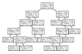
entropy_deci=DecisionTreeClassifier(criterion='entropy',max_depth=5,min_samples_leaf=3,random_state=100)
entropy_deci.fit(X_train,Y_train)
DecisionTreeClassifier(criterion='entropy', max_depth=5, min_samples_leaf=3,
                       random_state=100)
y_pred_entropy=entropy_deci.predict(X_test)
confusion_matrix(Y_test,y_pred_entropy)
array([[10,  2],
       [ 0, 12]])
print(classification_report(Y_test,y_pred_entropy))
              precision    recall  f1-score   support

           1       1.00      0.83      0.91        12
           2       0.86      1.00      0.92        12

    accuracy                           0.92        24
   macro avg       0.93      0.92      0.92        24
weighted avg       0.93      0.92      0.92        24
from sklearn import tree
tree.plot_tree(giniindex)
[Text(0.47619047619047616, 0.9166666666666666, 'X[1] <= 91.5\ngini = 0.491\nsamples = 92\nvalue = [40, 52]'),
 Text(0.21428571428571427, 0.75, 'X[2] <= 3.793\ngini = 0.432\nsamples = 38\nvalue = [26, 12]'),
 Text(0.09523809523809523, 0.5833333333333334, 'X[6] <= 13.163\ngini = 0.375\nsamples = 8\nvalue = [2, 6]'),
 Text(0.047619047619047616, 0.4166666666666667, 'gini = 0.5\nsamples = 4\nvalue = [2, 2]'),
 Text(0.14285714285714285, 0.4166666666666667, 'gini = 0.0\nsamples = 4\nvalue = [0, 4]'),
 Text(0.3333333333333333, 0.5833333333333334, 'X[6] <= 14.227\ngini = 0.32\nsamples = 30\nvalue = [24, 6]'),
 Text(0.23809523809523808, 0.4166666666666667, 'X[2] <= 14.391\ngini = 0.111\nsamples = 17\nvalue = [16, 1]'),
 Text(0.19047619047619047, 0.25, 'gini = 0.0\nsamples = 14\nvalue = [14, 0]'),
 Text(0.2857142857142857, 0.25, 'gini = 0.444\nsamples = 3\nvalue = [2, 1]'),
 Text(0.42857142857142855, 0.4166666666666667, 'X[0] <= 31.124\ngini = 0.473\nsamples = 13\nvalue = [8, 5]'),
 Text(0.38095238095238093, 0.25, 'X[5] <= 7.537\ngini = 0.278\nsamples = 6\nvalue = [1, 5]'),
 Text(0.3333333333333333, 0.08333333333333333, 'gini = 0.0\nsamples = 3\nvalue = [0, 3]'),
 Text(0.42857142857142855, 0.08333333333333333, 'gini = 0.444\nsamples = 3\nvalue = [1, 2]'),
 Text(0.47619047619047616, 0.25, 'gini = 0.0\nsamples = 7\nvalue = [7, 0]'),
 Text(0.7380952380952381, 0.75, 'X[4] <= 7.24\ngini = 0.384\nsamples = 54\nvalue = [14, 40]'),
 Text(0.6904761904761905, 0.5833333333333334, 'gini = 0.0\nsamples = 3\nvalue = [3, 0]'),
 Text(0.7857142857142857, 0.5833333333333334, 'X[4] <= 55.591\ngini = 0.338\nsamples = 51\nvalue = [11, 40]'),
 Text(0.6666666666666666, 0.4166666666666667, 'X[6] <= 11.927\ngini = 0.268\nsamples = 44\nvalue = [7, 37]'),
 Text(0.5714285714285714, 0.25, 'X[6] <= 8.31\ngini = 0.386\nsamples = 23\nvalue = [6, 17]'),
 Text(0.5238095238095238, 0.08333333333333333, 'gini = 0.153\nsamples = 12\nvalue = [1, 11]'),
 Text(0.6190476190476191, 0.08333333333333333, 'gini = 0.496\nsamples = 11\nvalue = [5, 6]'),
 Text(0.7619047619047619, 0.25, 'X[5] <= 3.924\ngini = 0.091\nsamples = 21\nvalue = [1, 20]'),
 Text(0.7142857142857143, 0.08333333333333333, 'gini = 0.444\nsamples = 3\nvalue = [1, 2]'),
 Text(0.8095238095238095, 0.08333333333333333, 'gini = 0.0\nsamples = 18\nvalue = [0, 18]'),
 Text(0.9047619047619048, 0.4166666666666667, 'X[5] <= 7.721\ngini = 0.49\nsamples = 7\nvalue = [4, 3]'),
 Text(0.8571428571428571, 0.25, 'gini = 0.0\nsamples = 3\nvalue = [3, 0]'),
 Text(0.9523809523809523, 0.25, 'gini = 0.375\nsamples = 4\nvalue = [1, 3]')]
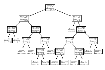
tree.plot_tree(entropy_deci)
[Text(0.5769230769230769, 0.9166666666666666, 'X[1] <= 91.5\nentropy = 0.988\nsamples = 92\nvalue = [40, 52]'),
 Text(0.38461538461538464, 0.75, 'X[0] <= 31.124\nentropy = 0.9\nsamples = 38\nvalue = [26, 12]'),
 Text(0.3076923076923077, 0.5833333333333334, 'X[6] <= 13.248\nentropy = 0.991\nsamples = 27\nvalue = [15, 12]'),
 Text(0.15384615384615385, 0.4166666666666667, 'X[2] <= 3.793\nentropy = 0.672\nsamples = 17\nvalue = [14, 3]'),
 Text(0.07692307692307693, 0.25, 'entropy = 1.0\nsamples = 4\nvalue = [2, 2]'),
 Text(0.23076923076923078, 0.25, 'X[2] <= 6.83\nentropy = 0.391\nsamples = 13\nvalue = [12, 1]'),
 Text(0.15384615384615385, 0.08333333333333333, 'entropy = 0.0\nsamples = 10\nvalue = [10, 0]'),
 Text(0.3076923076923077, 0.08333333333333333, 'entropy = 0.918\nsamples = 3\nvalue = [2, 1]'),
 Text(0.46153846153846156, 0.4166666666666667, 'X[4] <= 28.041\nentropy = 0.469\nsamples = 10\nvalue = [1, 9]'),
 Text(0.38461538461538464, 0.25, 'entropy = 0.0\nsamples = 7\nvalue = [0, 7]'),
 Text(0.5384615384615384, 0.25, 'entropy = 0.918\nsamples = 3\nvalue = [1, 2]'),
 Text(0.46153846153846156, 0.5833333333333334, 'entropy = 0.0\nsamples = 11\nvalue = [11, 0]'),
 Text(0.7692307692307693, 0.75, 'X[4] <= 7.24\nentropy = 0.826\nsamples = 54\nvalue = [14, 40]'),
 Text(0.6923076923076923, 0.5833333333333334, 'entropy = 0.0\nsamples = 3\nvalue = [3, 0]'),
 Text(0.8461538461538461, 0.5833333333333334, 'X[1] <= 111.0\nentropy = 0.752\nsamples = 51\nvalue = [11, 40]'),
 Text(0.7692307692307693, 0.4166666666666667, 'X[4] <= 63.703\nentropy = 0.839\nsamples = 41\nvalue = [11, 30]'),
 Text(0.6923076923076923, 0.25, 'X[6] <= 20.361\nentropy = 0.742\nsamples = 38\nvalue = [8, 30]'),
 Text(0.6153846153846154, 0.08333333333333333, 'entropy = 0.863\nsamples = 28\nvalue = [8, 20]'),
 Text(0.7692307692307693, 0.08333333333333333, 'entropy = 0.0\nsamples = 10\nvalue = [0, 10]'),
 Text(0.8461538461538461, 0.25, 'entropy = 0.0\nsamples = 3\nvalue = [3, 0]'),
 Text(0.9230769230769231, 0.4166666666666667, 'entropy = 0.0\nsamples = 10\nvalue = [0, 10]')]
Tugas 7 : CREDIT RISK MODELING#
# Import library yang diperlukan
import pandas as pd
import numpy as np
from sklearn import preprocessing
# Membaca dataset kredit
dataset = pd.read_csv("https://raw.githubusercontent.com/Rosita19/datamining/main/credit_score.csv")
# Menampilkan data skor kredit
dataset.head()
| Unnamed: 0 | kode_kontrak | pendapatan_setahun_juta | kpr_aktif | durasi_pinjaman_bulan | jumlah_tanggungan | rata_rata_overdue | risk_rating | |
|---|---|---|---|---|---|---|---|---|
| 0 | 1 | AGR-000001 | 295 | YA | 48 | 5 | 61 - 90 days | 4 |
| 1 | 2 | AGR-000011 | 271 | YA | 36 | 5 | 61 - 90 days | 4 |
| 2 | 3 | AGR-000030 | 159 | TIDAK | 12 | 0 | 0 - 30 days | 1 |
| 3 | 4 | AGR-000043 | 210 | YA | 12 | 3 | 46 - 60 days | 3 |
| 4 | 5 | AGR-000049 | 165 | TIDAK | 36 | 0 | 31 - 45 days | 2 |
# Melihat jumlah baris dan kolom
dataset.shape
(900, 8)
Mengubah data kategorikal menjadi numerik menggunakan teknik One-Hot Encoding
# Mengambil kolom kpr aktif dan mentranformasikan menggunakan one-hot encoding
df_kpr_aktif=pd.get_dummies(dataset['kpr_aktif'])
df_kpr_aktif.head()
| TIDAK | YA | |
|---|---|---|
| 0 | 0 | 1 |
| 1 | 0 | 1 |
| 2 | 1 | 0 |
| 3 | 0 | 1 |
| 4 | 1 | 0 |
# Mengambil kolom rata-rata overdue mentranformasi menggunakan one-hot encoding
rata_rata_overdue=pd.get_dummies(dataset['rata_rata_overdue'])
rata_rata_overdue.head()
| 0 - 30 days | 31 - 45 days | 46 - 60 days | 61 - 90 days | > 90 days | |
|---|---|---|---|---|---|
| 0 | 0 | 0 | 0 | 1 | 0 |
| 1 | 0 | 0 | 0 | 1 | 0 |
| 2 | 1 | 0 | 0 | 0 | 0 |
| 3 | 0 | 0 | 1 | 0 | 0 |
| 4 | 0 | 1 | 0 | 0 | 0 |
# Mengambil data numeric
numeric = pd.DataFrame(dataset, columns = ['kode_kontrak','pendapatan_setahun_juta','durasi_pinjaman_bulan','jumlah_tanggungan','risk_rating'])
numeric.head()
| kode_kontrak | pendapatan_setahun_juta | durasi_pinjaman_bulan | jumlah_tanggungan | risk_rating | |
|---|---|---|---|---|---|
| 0 | AGR-000001 | 295 | 48 | 5 | 4 |
| 1 | AGR-000011 | 271 | 36 | 5 | 4 |
| 2 | AGR-000030 | 159 | 12 | 0 | 1 |
| 3 | AGR-000043 | 210 | 12 | 3 | 3 |
| 4 | AGR-000049 | 165 | 36 | 0 | 2 |
# Menampilkan gabungan beberapa kolom yang telah diproses
dataset_baru = pd.concat([numeric, df_kpr_aktif, rata_rata_overdue], axis=1)
dataset_baru.head()
| kode_kontrak | pendapatan_setahun_juta | durasi_pinjaman_bulan | jumlah_tanggungan | risk_rating | TIDAK | YA | 0 - 30 days | 31 - 45 days | 46 - 60 days | 61 - 90 days | > 90 days | |
|---|---|---|---|---|---|---|---|---|---|---|---|---|
| 0 | AGR-000001 | 295 | 48 | 5 | 4 | 0 | 1 | 0 | 0 | 0 | 1 | 0 |
| 1 | AGR-000011 | 271 | 36 | 5 | 4 | 0 | 1 | 0 | 0 | 0 | 1 | 0 |
| 2 | AGR-000030 | 159 | 12 | 0 | 1 | 1 | 0 | 1 | 0 | 0 | 0 | 0 |
| 3 | AGR-000043 | 210 | 12 | 3 | 3 | 0 | 1 | 0 | 0 | 1 | 0 | 0 |
| 4 | AGR-000049 | 165 | 36 | 0 | 2 | 1 | 0 | 0 | 1 | 0 | 0 | 0 |
# Mengambil kolom selain kode_kontrak dan risk_rating dan melakukan normalisasi data
normalisasi = dataset_baru.drop(["kode_kontrak", "risk_rating"], axis=1)
Normalisasi data menggunakan Min Max
from sklearn.preprocessing import MinMaxScaler
# Melakukan scaler fitur
scaler = MinMaxScaler()
model =scaler.fit(normalisasi)
scaled_data=model.transform(normalisasi)
# Menampilkan scaler fitur
print(scaled_data)
[[0.97826087 1.         0.83333333 ... 0.         1.         0.        ]
 [0.87391304 0.66666667 0.83333333 ... 0.         1.         0.        ]
 [0.38695652 0.         0.         ... 0.         0.         0.        ]
 ...
 [0.4173913  0.33333333 0.33333333 ... 0.         0.         0.        ]
 [0.54782609 1.         0.         ... 0.         0.         0.        ]
 [0.5826087  0.33333333 0.33333333 ... 0.         0.         0.        ]]
# Menampilkan data normalisasi dari min max
namakolom = normalisasi.columns.values
dataMinMax = pd.DataFrame(scaled_data, columns=namakolom)
dataMinMax.head()
| pendapatan_setahun_juta | durasi_pinjaman_bulan | jumlah_tanggungan | TIDAK | YA | 0 - 30 days | 31 - 45 days | 46 - 60 days | 61 - 90 days | > 90 days | |
|---|---|---|---|---|---|---|---|---|---|---|
| 0 | 0.978261 | 1.000000 | 0.833333 | 0.0 | 1.0 | 0.0 | 0.0 | 0.0 | 1.0 | 0.0 |
| 1 | 0.873913 | 0.666667 | 0.833333 | 0.0 | 1.0 | 0.0 | 0.0 | 0.0 | 1.0 | 0.0 |
| 2 | 0.386957 | 0.000000 | 0.000000 | 1.0 | 0.0 | 1.0 | 0.0 | 0.0 | 0.0 | 0.0 |
| 3 | 0.608696 | 0.000000 | 0.500000 | 0.0 | 1.0 | 0.0 | 0.0 | 1.0 | 0.0 | 0.0 |
| 4 | 0.413043 | 0.666667 | 0.000000 | 1.0 | 0.0 | 0.0 | 1.0 | 0.0 | 0.0 | 0.0 |
Normalisasi dengan Min=1 dan Max=2
# Min Max Scale dengan Min = 1 dan Max =2
scaler = MinMaxScaler(feature_range=(1,2))
model =scaler.fit(normalisasi)
scaled_data2=model.transform(normalisasi)
# Menampilkan skala fitur
print(scaled_data2)
[[1.97826087 2.         1.83333333 ... 1.         2.         1.        ]
 [1.87391304 1.66666667 1.83333333 ... 1.         2.         1.        ]
 [1.38695652 1.         1.         ... 1.         1.         1.        ]
 ...
 [1.4173913  1.33333333 1.33333333 ... 1.         1.         1.        ]
 [1.54782609 2.         1.         ... 1.         1.         1.        ]
 [1.5826087  1.33333333 1.33333333 ... 1.         1.         1.        ]]
# Menampilkan data normalisasi dari min=1 dan max=2
dataMinMax2 = pd.DataFrame(scaled_data2, columns=normalisasi.columns.values)
dataMinMax2.head()
| pendapatan_setahun_juta | durasi_pinjaman_bulan | jumlah_tanggungan | TIDAK | YA | 0 - 30 days | 31 - 45 days | 46 - 60 days | 61 - 90 days | > 90 days | |
|---|---|---|---|---|---|---|---|---|---|---|
| 0 | 1.978261 | 2.000000 | 1.833333 | 1.0 | 2.0 | 1.0 | 1.0 | 1.0 | 2.0 | 1.0 |
| 1 | 1.873913 | 1.666667 | 1.833333 | 1.0 | 2.0 | 1.0 | 1.0 | 1.0 | 2.0 | 1.0 |
| 2 | 1.386957 | 1.000000 | 1.000000 | 2.0 | 1.0 | 2.0 | 1.0 | 1.0 | 1.0 | 1.0 |
| 3 | 1.608696 | 1.000000 | 1.500000 | 1.0 | 2.0 | 1.0 | 1.0 | 2.0 | 1.0 | 1.0 |
| 4 | 1.413043 | 1.666667 | 1.000000 | 2.0 | 1.0 | 1.0 | 2.0 | 1.0 | 1.0 | 1.0 |
Normalisasi dengan Z Score
# Melakukan normalisasi dengan z score atau standarscale
from sklearn.preprocessing import StandardScaler
scaler = StandardScaler()
model = (scaler.fit(normalisasi))
data_mean = (scaler.mean_)
scale_data = (scaler.transform(normalisasi))
print(scale_data)
[[ 2.54041987  1.32217147  1.03062105 ... -0.6912543   2.54950976
  -0.35949218]
 [ 2.07740679  0.4439764   1.03062105 ... -0.6912543   2.54950976
  -0.35949218]
 [-0.08332092 -1.31241375 -1.46147714 ... -0.6912543  -0.39223227
  -0.35949218]
 ...
 [ 0.05172456 -0.43421867 -0.46463786 ... -0.6912543  -0.39223227
  -0.35949218]
 [ 0.63049091  1.32217147 -1.46147714 ... -0.6912543  -0.39223227
  -0.35949218]
 [ 0.78482861 -0.43421867 -0.46463786 ... -0.6912543  -0.39223227
  -0.35949218]]
# Menampilkan data normalisasi dari z score
dataZScale = pd.DataFrame(scale_data, columns=normalisasi.columns.values)
dataZScale.head()
| pendapatan_setahun_juta | durasi_pinjaman_bulan | jumlah_tanggungan | TIDAK | YA | 0 - 30 days | 31 - 45 days | 46 - 60 days | 61 - 90 days | > 90 days | |
|---|---|---|---|---|---|---|---|---|---|---|
| 0 | 2.540420 | 1.322171 | 1.030621 | -0.868554 | 0.868554 | -0.580772 | -0.463222 | -0.691254 | 2.549510 | -0.359492 |
| 1 | 2.077407 | 0.443976 | 1.030621 | -0.868554 | 0.868554 | -0.580772 | -0.463222 | -0.691254 | 2.549510 | -0.359492 |
| 2 | -0.083321 | -1.312414 | -1.461477 | 1.151339 | -1.151339 | 1.721847 | -0.463222 | -0.691254 | -0.392232 | -0.359492 |
| 3 | 0.900582 | -1.312414 | 0.033782 | -0.868554 | 0.868554 | -0.580772 | -0.463222 | 1.446646 | -0.392232 | -0.359492 |
| 4 | 0.032432 | 0.443976 | -1.461477 | 1.151339 | -1.151339 | -0.580772 | 2.158791 | -0.691254 | -0.392232 | -0.359492 |
Menggabungkan kolom yang telah dinormalisasi
# Mengambil kolom kode kontak dan risk rating
data_kontrak_risk= pd.DataFrame(dataset, columns=['kode_kontrak','risk_rating'])
# Menggabungkan kolom yang sudah dinormalisasi dan data sebelumnya
kredit_min_max = pd.concat([data_kontrak_risk, dataMinMax], axis=1)
kredit_min_max.head()
| kode_kontrak | risk_rating | pendapatan_setahun_juta | durasi_pinjaman_bulan | jumlah_tanggungan | TIDAK | YA | 0 - 30 days | 31 - 45 days | 46 - 60 days | 61 - 90 days | > 90 days | |
|---|---|---|---|---|---|---|---|---|---|---|---|---|
| 0 | AGR-000001 | 4 | 0.978261 | 1.000000 | 0.833333 | 0.0 | 1.0 | 0.0 | 0.0 | 0.0 | 1.0 | 0.0 |
| 1 | AGR-000011 | 4 | 0.873913 | 0.666667 | 0.833333 | 0.0 | 1.0 | 0.0 | 0.0 | 0.0 | 1.0 | 0.0 |
| 2 | AGR-000030 | 1 | 0.386957 | 0.000000 | 0.000000 | 1.0 | 0.0 | 1.0 | 0.0 | 0.0 | 0.0 | 0.0 |
| 3 | AGR-000043 | 3 | 0.608696 | 0.000000 | 0.500000 | 0.0 | 1.0 | 0.0 | 0.0 | 1.0 | 0.0 | 0.0 |
| 4 | AGR-000049 | 2 | 0.413043 | 0.666667 | 0.000000 | 1.0 | 0.0 | 0.0 | 1.0 | 0.0 | 0.0 | 0.0 |
# Menggabungkan kolom yang sudah dinormalisasi dan data sebelumnya
kredit_min1_max2 = pd.concat([data_kontrak_risk, dataMinMax2], axis=1)
kredit_min1_max2.head()
| kode_kontrak | risk_rating | pendapatan_setahun_juta | durasi_pinjaman_bulan | jumlah_tanggungan | TIDAK | YA | 0 - 30 days | 31 - 45 days | 46 - 60 days | 61 - 90 days | > 90 days | |
|---|---|---|---|---|---|---|---|---|---|---|---|---|
| 0 | AGR-000001 | 4 | 1.978261 | 2.000000 | 1.833333 | 1.0 | 2.0 | 1.0 | 1.0 | 1.0 | 2.0 | 1.0 |
| 1 | AGR-000011 | 4 | 1.873913 | 1.666667 | 1.833333 | 1.0 | 2.0 | 1.0 | 1.0 | 1.0 | 2.0 | 1.0 |
| 2 | AGR-000030 | 1 | 1.386957 | 1.000000 | 1.000000 | 2.0 | 1.0 | 2.0 | 1.0 | 1.0 | 1.0 | 1.0 |
| 3 | AGR-000043 | 3 | 1.608696 | 1.000000 | 1.500000 | 1.0 | 2.0 | 1.0 | 1.0 | 2.0 | 1.0 | 1.0 |
| 4 | AGR-000049 | 2 | 1.413043 | 1.666667 | 1.000000 | 2.0 | 1.0 | 1.0 | 2.0 | 1.0 | 1.0 | 1.0 |
# Menggabungkan kolom yang sudah dinormalisasi Z score dan data sebelumnya
kredit_Zscore = pd.concat([data_kontrak_risk, dataZScale], axis=1)
kredit_Zscore.head()
| kode_kontrak | risk_rating | pendapatan_setahun_juta | durasi_pinjaman_bulan | jumlah_tanggungan | TIDAK | YA | 0 - 30 days | 31 - 45 days | 46 - 60 days | 61 - 90 days | > 90 days | |
|---|---|---|---|---|---|---|---|---|---|---|---|---|
| 0 | AGR-000001 | 4 | 2.540420 | 1.322171 | 1.030621 | -0.868554 | 0.868554 | -0.580772 | -0.463222 | -0.691254 | 2.549510 | -0.359492 |
| 1 | AGR-000011 | 4 | 2.077407 | 0.443976 | 1.030621 | -0.868554 | 0.868554 | -0.580772 | -0.463222 | -0.691254 | 2.549510 | -0.359492 |
| 2 | AGR-000030 | 1 | -0.083321 | -1.312414 | -1.461477 | 1.151339 | -1.151339 | 1.721847 | -0.463222 | -0.691254 | -0.392232 | -0.359492 |
| 3 | AGR-000043 | 3 | 0.900582 | -1.312414 | 0.033782 | -0.868554 | 0.868554 | -0.580772 | -0.463222 | 1.446646 | -0.392232 | -0.359492 |
| 4 | AGR-000049 | 2 | 0.032432 | 0.443976 | -1.461477 | 1.151339 | -1.151339 | -0.580772 | 2.158791 | -0.691254 | -0.392232 | -0.359492 |
Membagi data menjadi data training dan melakukan pengujian di Min Max
# Mengambil kelas dan fitur dari dataset
# fiturnya
X_min_max = kredit_min_max.iloc[:,2:12].values
# classnya
y_min_max = kredit_min_max.iloc[:,1].values
# Membagi data menjadi data training dan data uji dengan data uji berjumlah 30%
from sklearn.model_selection import train_test_split
X_trainn_min_max, X_testn_min_max, y_trainn_min_max, y_testn_min_max = train_test_split(X_min_max, y_min_max, test_size=0.30, random_state=0, stratify=y_min_max)
Membagi data menjadi training dan uji di min=1 dan max=2
# Mengambil kelas dan fitur dari dataset
# fiturnya
X_min1_max2 = kredit_min1_max2.iloc[:,2:12].values
# classnya
y_min1_max2 = kredit_min1_max2.iloc[:,1].values
# Membagi data menjadi data training dan data uji dengan data uji berjumlah 30%
X_trainn_min1_max2, X_testn_min1_max2, y_trainn_min1_max2, y_testn_min1_max2 = train_test_split(X_min1_max2, y_min1_max2, test_size=0.30, random_state=0, stratify=y_min1_max2)
Membagi data menjadi data training dan uji di Z Score
# Mengambil kelas dan fitur dari dataset
# fiturnya
X_Zscore = kredit_Zscore.iloc[:,2:12].values
# classnya
y_Zscore = kredit_Zscore.iloc[:,1].values
# Membagi data menjadi data training dan data uji dengan data uji berjumlah 30%
X_trainn_Zscore, X_testn_Zscore, y_trainn_Zscore, y_testn_Zscore = train_test_split(X_Zscore, y_Zscore, test_size=0.30, random_state=0, stratify=y_Zscore)
Naive Bayes
# Melakukan import library yang diperlukan
from sklearn.metrics import make_scorer, accuracy_score,precision_score
from sklearn.metrics import accuracy_score ,precision_score,recall_score,f1_score
from sklearn.metrics import confusion_matrix
from sklearn.model_selection import KFold,train_test_split,cross_val_score
from sklearn.naive_bayes import GaussianNB
from sklearn.model_selection import train_test_split
Naive Bayes dengan normalisasi Min Max
# Menghitung akurasi presisi dari naive bayes dengan normalisasi min max
gaussian = GaussianNB()
gaussian.fit(X_trainn_min_max, y_trainn_min_max)
Y_predn_min_max = gaussian.predict(X_testn_min_max)
accuracy_n_min_max=round(accuracy_score(y_testn_min_max,Y_predn_min_max)* 100, 2)
acc_gaussian = round(gaussian.score(X_trainn_min_max, y_trainn_min_max) * 100, 2)

confusion_m_min_max = confusion_matrix(y_testn_min_max, Y_predn_min_max)
accuracy_n_min_max = accuracy_score(y_testn_min_max,Y_predn_min_max)
precision_n_min_max =precision_score(y_testn_min_max, Y_predn_min_max,average='micro')
recall_n_min_max =  recall_score(y_testn_min_max, Y_predn_min_max,average='micro')
f1_n_min_max = f1_score(y_testn_min_max,Y_predn_min_max,average='micro')
print('Confusion matrix untuk Naive Bayes\n',confusion_m_min_max)
print('Akurasi Naive Bayes: %.3f' %accuracy_n_min_max)
print('Precision Naive Bayes: %.3f' %precision_n_min_max)
print('Recall Naive Bayes: %.3f' %recall_n_min_max)
print('f1-score Naive Bayes : %.3f' %f1_n_min_max)
Confusion matrix untuk Naive Bayes
 [[68  0  0  0  0]
 [ 0 48  0  0  0]
 [ 0  0 87  0  0]
 [ 0  0  0 36  0]
 [ 0  0  0  0 31]]
Akurasi Naive Bayes: 1.000
Precision Naive Bayes: 1.000
Recall Naive Bayes: 1.000
f1-score Naive Bayes : 1.000
Naive Bayes dengan normalisasi Min=1 dan Max=2
# Menghitung akurasi presisi dari naive bayes dengan normalisasi min=1 dan max=2
gaussian = GaussianNB()
gaussian.fit(X_trainn_min1_max2, y_trainn_min1_max2)
Y_predn_min1_max2 = gaussian.predict(X_testn_min1_max2)
accuracy_n_min1_max2=round(accuracy_score(y_testn_min1_max2,Y_predn_min1_max2)* 100, 2)
acc_gaussian = round(gaussian.score(X_trainn_min1_max2, y_trainn_min1_max2) * 100, 2)

confusion_m_min1_max2 = confusion_matrix(y_testn_min1_max2, Y_predn_min1_max2)
accuracy_n_min1_max2 = accuracy_score(y_testn_min1_max2,Y_predn_min1_max2)
precision_n_min1_max2 =precision_score(y_testn_min1_max2, Y_predn_min1_max2,average='micro')
recall_n_min1_max2 =  recall_score(y_testn_min1_max2, Y_predn_min1_max2,average='micro')
f1_n_min1_max2 = f1_score(y_testn_min1_max2,Y_predn_min1_max2,average='micro')
print('Confusion matrix untuk Naive Bayes\n',confusion_m_min1_max2)
print('Akurasi Naive Bayes: %.3f' %accuracy_n_min1_max2)
print('Precision Naive Bayes: %.3f' %precision_n_min1_max2)
print('Recall Naive Bayes: %.3f' %recall_n_min1_max2)
print('f1-score Naive Bayes : %.3f' %f1_n_min1_max2)
Confusion matrix untuk Naive Bayes
 [[68  0  0  0  0]
 [ 0 48  0  0  0]
 [ 0  0 87  0  0]
 [ 0  0  0 36  0]
 [ 0  0  0  0 31]]
Akurasi Naive Bayes: 1.000
Precision Naive Bayes: 1.000
Recall Naive Bayes: 1.000
f1-score Naive Bayes : 1.000
Naive Bayes dengan normalisasi Z Score
# Menghitung akurasi presisi dari naive bayes dengan normalisasi z score
gaussian = GaussianNB()
gaussian.fit(X_trainn_Zscore, y_trainn_Zscore)
Y_predn_Zscore = gaussian.predict(X_testn_Zscore)
accuracy_n_Zscore=round(accuracy_score(y_testn_Zscore,Y_predn_Zscore)* 100, 2)
acc_gaussian = round(gaussian.score(X_trainn_Zscore, y_trainn_Zscore) * 100, 2)

confusion_m_Zscore = confusion_matrix(y_testn_Zscore, Y_predn_Zscore)
accuracy_n_Zscore = accuracy_score(y_testn_Zscore,Y_predn_Zscore)
precision_n_Zscore =precision_score(y_testn_Zscore, Y_predn_Zscore,average='micro')
recall_n_Zscore =  recall_score(y_testn_Zscore, Y_predn_Zscore,average='micro')
f1_n_Zscore = f1_score(y_testn_Zscore,Y_predn_Zscore,average='micro')
print('Confusion matrix untuk Naive Bayes\n',confusion_m_Zscore)
print('Akurasi Naive Bayes: %.3f' %accuracy_n_Zscore)
print('Precision Naive Bayes: %.3f' %precision_n_Zscore)
print('Recall Naive Bayes: %.3f' %recall_n_Zscore)
print('f1-score Naive Bayes : %.3f' %f1_n_Zscore)
Confusion matrix untuk Naive Bayes
 [[68  0  0  0  0]
 [ 0 48  0  0  0]
 [ 0  0 87  0  0]
 [ 0  0  0 36  0]
 [ 0  0  0  0 31]]
Akurasi Naive Bayes: 1.000
Precision Naive Bayes: 1.000
Recall Naive Bayes: 1.000
f1-score Naive Bayes : 1.000
KNN
KNN dengan normalisasi Min dan Max
# Menghitung akurasi dari KNN dengan normalisasi min dan max
from sklearn.neighbors import KNeighborsClassifier
neigh = KNeighborsClassifier(n_neighbors=3)
neigh.fit(X_trainn_min_max, y_trainn_min_max)

acc_knn = round(neigh.score(X_trainn_min_max, y_trainn_min_max) * 100, 2)
print("Akurasi KNN :",acc_knn)
Akurasi KNN : 99.68
KNN dengan normalisasi Min=1 dan Max=2
# Menghitung akurasi dari KNN dengan normalisasi min=1 dan max=2
from sklearn.neighbors import KNeighborsClassifier
neigh = KNeighborsClassifier(n_neighbors=3)
neigh.fit(X_trainn_min1_max2, y_trainn_min1_max2)

acc_knn = round(neigh.score(X_trainn_min1_max2, y_trainn_min1_max2) * 100, 2)
print("Akurasi KNN :",acc_knn)
Akurasi KNN : 99.68
KNN dengan normalisasi Z Score
# Menghitung akurasi dari KNN dengan normalisasi z score
from sklearn.neighbors import KNeighborsClassifier
neigh = KNeighborsClassifier(n_neighbors=3)
neigh.fit(X_trainn_Zscore, y_trainn_Zscore)

acc_knn = round(neigh.score(X_trainn_Zscore, y_trainn_Zscore) * 100, 2)
print("Akurasi KNN :",acc_knn)
Akurasi KNN : 100.0
Decision Treee
# Import library yang diperlukan pada decision tree
from sklearn.metrics import accuracy_score
from sklearn import tree
from sklearn import metrics
from matplotlib import pyplot as plt
Decision Tree dengan normalisasi Min dan max
# Menghitung akurasi dengan menggunakan gini indek dengan normalisasi min max
clf = tree.DecisionTreeClassifier(criterion="gini")
clf = clf.fit(X_trainn_min_max, y_trainn_min_max)

y_predn_min_max = clf.predict(X_testn_min_max)
print("Accuracy_Decision Tree :",metrics.accuracy_score(y_testn_min_max,y_predn_min_max))
Accuracy_Decision Tree : 1.0
Decision Tree dengan normalisasi Min=1 dan Max=2
# Menghitung akurasi dengan menggunakan gini indek dengan normalisasi Min=1 dan Max=2
clf = tree.DecisionTreeClassifier(criterion="gini")
clf = clf.fit(X_trainn_min1_max2, y_trainn_min1_max2)

y_predn_min1_max2 = clf.predict(X_testn_min1_max2)
print("Accuracy_Decision Tree :",metrics.accuracy_score(y_testn_min1_max2, y_predn_min1_max2))
Accuracy_Decision Tree : 1.0
Decision Tree dengan normalisasi Z Score
# Menghitung akurasi dengan menggunakan gini indek dengan normalisasi Z Score
clf = tree.DecisionTreeClassifier(criterion="gini")
clf = clf.fit(X_trainn_Zscore, y_trainn_Zscore)

y_predn_Zscore = clf.predict(X_testn_Zscore)
print("Accuracy_Decision Tree :",metrics.accuracy_score(y_testn_Zscore,y_predn_Zscore))
Accuracy_Decision Tree : 1.0
# gambar bentuk decision tree
plt.figure(figsize=(15,15))
#Membuat plot
a = tree.plot_tree(clf,
                   rounded = True,
                   filled = True,
                   fontsize=8)
#Menampilkan plot
plt.show()
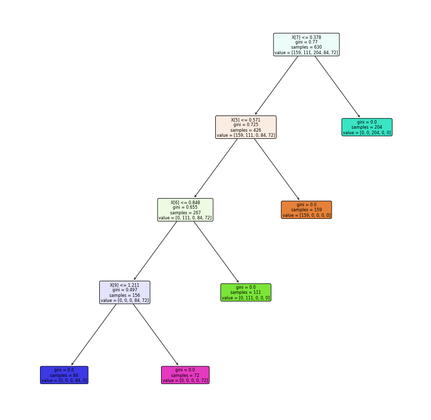
Tugas 8 : Bagging Esamble Learning#
# Import library yang diperlukan
from sklearn.ensemble import BaggingClassifier
from sklearn.neighbors import KNeighborsClassifier
from sklearn.tree import DecisionTreeClassifier
clf = BaggingClassifier(base_estimator=DecisionTreeClassifier(),n_estimators=10, random_state=0).fit(X_trainn_min_max, y_trainn_min_max)
rsb = clf.predict(X_testn_min_max)
b = ['Decision Tree']
Tree = pd.DataFrame(rsb,columns = b)
X_testn_min_max.shape
(270, 10)
K = 10
clf = BaggingClassifier(base_estimator=KNeighborsClassifier(n_neighbors = K),n_estimators=10, random_state=0).fit(X_trainn_min_max, y_trainn_min_max)
rsa = clf.predict(X_testn_min_max)
a = ['KNN']
KNN = pd.DataFrame(rsa,columns = a)
clf = BaggingClassifier(base_estimator=GaussianNB(),n_estimators=10, random_state=0).fit(X_trainn_min_max, y_trainn_min_max)
rsc = clf.predict(X_testn_min_max)
c = ['Naive Bayes']
Bayes = pd.DataFrame(rsc,columns = c)
Result = pd.concat([Tree, KNN,Bayes], axis=1)
Result
| Decision Tree | KNN | Naive Bayes | |
|---|---|---|---|
| 0 | 4 | 4 | 4 |
| 1 | 3 | 3 | 3 |
| 2 | 1 | 1 | 1 |
| 3 | 3 | 3 | 3 |
| 4 | 3 | 3 | 3 |
| ... | ... | ... | ... |
| 265 | 1 | 1 | 1 |
| 266 | 4 | 4 | 4 |
| 267 | 1 | 1 | 1 |
| 268 | 3 | 3 | 3 |
| 269 | 3 | 3 | 3 |
270 rows × 3 columns
bagging_accuracy1 = round(100 * accuracy_score(y_testn_min_max, Bayes), 2)
bagging_accuracy2 = round(100 * accuracy_score(y_testn_min_max, Tree), 2)
bagging_accuracy3 = round(100 * accuracy_score(y_testn_min_max, KNN), 2)
print('The accuracy of this model is Bagging Naive Bayes {} %.'.format(bagging_accuracy1))
print('The accuracy of this model is Bagging Decision Tree {} %.'.format(bagging_accuracy2))
print('The accuracy of this model is Bagging kNN {} %.'.format(bagging_accuracy3))
The accuracy of this model is Bagging Naive Bayes 100.0 %.
The accuracy of this model is Bagging Decision Tree 100.0 %.
The accuracy of this model is Bagging kNN 99.63 %.
UAS#
import pandas as pd
df = pd.read_csv("https://raw.githubusercontent.com/Rosita19/datamining/main/credit_score.csv")
df
| Unnamed: 0 | kode_kontrak | pendapatan_setahun_juta | kpr_aktif | durasi_pinjaman_bulan | jumlah_tanggungan | rata_rata_overdue | risk_rating | |
|---|---|---|---|---|---|---|---|---|
| 0 | 1 | AGR-000001 | 295 | YA | 48 | 5 | 61 - 90 days | 4 |
| 1 | 2 | AGR-000011 | 271 | YA | 36 | 5 | 61 - 90 days | 4 |
| 2 | 3 | AGR-000030 | 159 | TIDAK | 12 | 0 | 0 - 30 days | 1 |
| 3 | 4 | AGR-000043 | 210 | YA | 12 | 3 | 46 - 60 days | 3 |
| 4 | 5 | AGR-000049 | 165 | TIDAK | 36 | 0 | 31 - 45 days | 2 |
| ... | ... | ... | ... | ... | ... | ... | ... | ... |
| 895 | 896 | AGR-010739 | 112 | YA | 48 | 5 | > 90 days | 5 |
| 896 | 897 | AGR-010744 | 120 | YA | 48 | 2 | 46 - 60 days | 3 |
| 897 | 898 | AGR-010758 | 166 | TIDAK | 24 | 2 | 0 - 30 days | 1 |
| 898 | 899 | AGR-010775 | 196 | TIDAK | 48 | 0 | 31 - 45 days | 2 |
| 899 | 900 | AGR-010790 | 204 | TIDAK | 24 | 2 | 0 - 30 days | 1 |
900 rows × 8 columns
#Exploration Data
df[["kode_kontrak", "pendapatan_setahun_juta", "kpr_aktif", "durasi_pinjaman_bulan", "jumlah_tanggungan", "rata_rata_overdue", "risk_rating"]].agg(['min','max'])
| kode_kontrak | pendapatan_setahun_juta | kpr_aktif | durasi_pinjaman_bulan | jumlah_tanggungan | rata_rata_overdue | risk_rating | |
|---|---|---|---|---|---|---|---|
| min | AGR-000001 | 70 | TIDAK | 12 | 0 | 0 - 30 days | 1 |
| max | AGR-010790 | 300 | YA | 48 | 6 | > 90 days | 5 |
df.shape
(900, 8)
preprocessing data#
from sklearn import preprocessing
le = preprocessing.LabelEncoder()
le.fit(y)
y = le.transform(y)
y
array([0, 0, 0, 0, 0, 0, 0, 0, 0, 0, 0, 0, 0, 0, 0, 0, 0, 0, 0, 0, 0, 0,
       0, 0, 0, 0, 0, 0, 0, 0, 0, 0, 0, 0, 0, 0, 0, 0, 0, 0, 0, 0, 0, 0,
       0, 0, 0, 0, 0, 0, 1, 1, 1, 1, 1, 1, 1, 1, 1, 1, 1, 1, 1, 1, 1, 1,
       1, 1, 1, 1, 1, 1, 1, 1, 1, 1, 1, 1, 1, 1, 1, 1, 1, 1, 1, 1, 1, 1,
       1, 1, 1, 1, 1, 1, 1, 1, 1, 1, 1, 1, 2, 2, 2, 2, 2, 2, 2, 2, 2, 2,
       2, 2, 2, 2, 2, 2, 2, 2, 2, 2, 2, 2, 2, 2, 2, 2, 2, 2, 2, 2, 2, 2,
       2, 2, 2, 2, 2, 2, 2, 2, 2, 2, 2, 2, 2, 2, 2, 2, 2, 2])
le.inverse_transform(y)
array([0, 0, 0, 0, 0, 0, 0, 0, 0, 0, 0, 0, 0, 0, 0, 0, 0, 0, 0, 0, 0, 0,
       0, 0, 0, 0, 0, 0, 0, 0, 0, 0, 0, 0, 0, 0, 0, 0, 0, 0, 0, 0, 0, 0,
       0, 0, 0, 0, 0, 0, 1, 1, 1, 1, 1, 1, 1, 1, 1, 1, 1, 1, 1, 1, 1, 1,
       1, 1, 1, 1, 1, 1, 1, 1, 1, 1, 1, 1, 1, 1, 1, 1, 1, 1, 1, 1, 1, 1,
       1, 1, 1, 1, 1, 1, 1, 1, 1, 1, 1, 1, 2, 2, 2, 2, 2, 2, 2, 2, 2, 2,
       2, 2, 2, 2, 2, 2, 2, 2, 2, 2, 2, 2, 2, 2, 2, 2, 2, 2, 2, 2, 2, 2,
       2, 2, 2, 2, 2, 2, 2, 2, 2, 2, 2, 2, 2, 2, 2, 2, 2, 2])
normalize data#
numeric = pd.DataFrame(df, columns = ['kode_kontrak','pendapatan_setahun_juta','durasi_pinjaman_bulan','jumlah_tanggungan','risk_rating'])
numeric.head()
| kode_kontrak | pendapatan_setahun_juta | durasi_pinjaman_bulan | jumlah_tanggungan | risk_rating | |
|---|---|---|---|---|---|
| 0 | AGR-000001 | 295 | 48 | 5 | 4 |
| 1 | AGR-000011 | 271 | 36 | 5 | 4 |
| 2 | AGR-000030 | 159 | 12 | 0 | 1 |
| 3 | AGR-000043 | 210 | 12 | 3 | 3 |
| 4 | AGR-000049 | 165 | 36 | 0 | 2 |
#UAS KU
READ DATA
import pandas as pd
df = pd.read_csv("https://raw.githubusercontent.com/Rosita19/datamining/main/healthcare-dataset-stroke-data.csv")
df
| id | gender | age | hypertension | heart_disease | ever_married | work_type | Residence_type | avg_glucose_level | bmi | smoking_status | stroke | |
|---|---|---|---|---|---|---|---|---|---|---|---|---|
| 0 | 9046 | Male | 67.0 | 0 | 1 | Yes | Private | Urban | 228.69 | 36.6 | formerly smoked | 1 |
| 1 | 51676 | Female | 61.0 | 0 | 0 | Yes | Self-employed | Rural | 202.21 | NaN | never smoked | 1 |
| 2 | 31112 | Male | 80.0 | 0 | 1 | Yes | Private | Rural | 105.92 | 32.5 | never smoked | 1 |
| 3 | 60182 | Female | 49.0 | 0 | 0 | Yes | Private | Urban | 171.23 | 34.4 | smokes | 1 |
| 4 | 1665 | Female | 79.0 | 1 | 0 | Yes | Self-employed | Rural | 174.12 | 24.0 | never smoked | 1 |
| ... | ... | ... | ... | ... | ... | ... | ... | ... | ... | ... | ... | ... |
| 5105 | 18234 | Female | 80.0 | 1 | 0 | Yes | Private | Urban | 83.75 | NaN | never smoked | 0 |
| 5106 | 44873 | Female | 81.0 | 0 | 0 | Yes | Self-employed | Urban | 125.20 | 40.0 | never smoked | 0 |
| 5107 | 19723 | Female | 35.0 | 0 | 0 | Yes | Self-employed | Rural | 82.99 | 30.6 | never smoked | 0 |
| 5108 | 37544 | Male | 51.0 | 0 | 0 | Yes | Private | Rural | 166.29 | 25.6 | formerly smoked | 0 |
| 5109 | 44679 | Female | 44.0 | 0 | 0 | Yes | Govt_job | Urban | 85.28 | 26.2 | Unknown | 0 |
5110 rows × 12 columns
Exploration Data
df
| id | gender | age | hypertension | heart_disease | ever_married | work_type | Residence_type | avg_glucose_level | bmi | smoking_status | stroke | |
|---|---|---|---|---|---|---|---|---|---|---|---|---|
| 0 | 9046 | Male | 67.0 | 0 | 1 | Yes | Private | Urban | 228.69 | 36.6 | formerly smoked | 1 |
| 1 | 51676 | Female | 61.0 | 0 | 0 | Yes | Self-employed | Rural | 202.21 | NaN | never smoked | 1 |
| 2 | 31112 | Male | 80.0 | 0 | 1 | Yes | Private | Rural | 105.92 | 32.5 | never smoked | 1 |
| 3 | 60182 | Female | 49.0 | 0 | 0 | Yes | Private | Urban | 171.23 | 34.4 | smokes | 1 |
| 4 | 1665 | Female | 79.0 | 1 | 0 | Yes | Self-employed | Rural | 174.12 | 24.0 | never smoked | 1 |
| ... | ... | ... | ... | ... | ... | ... | ... | ... | ... | ... | ... | ... |
| 5105 | 18234 | Female | 80.0 | 1 | 0 | Yes | Private | Urban | 83.75 | NaN | never smoked | 0 |
| 5106 | 44873 | Female | 81.0 | 0 | 0 | Yes | Self-employed | Urban | 125.20 | 40.0 | never smoked | 0 |
| 5107 | 19723 | Female | 35.0 | 0 | 0 | Yes | Self-employed | Rural | 82.99 | 30.6 | never smoked | 0 |
| 5108 | 37544 | Male | 51.0 | 0 | 0 | Yes | Private | Rural | 166.29 | 25.6 | formerly smoked | 0 |
| 5109 | 44679 | Female | 44.0 | 0 | 0 | Yes | Govt_job | Urban | 85.28 | 26.2 | Unknown | 0 |
5110 rows × 12 columns
df[["gender", "age", "hypertension", "heart_disease", "ever_married", "work_type", "Residence_type", "avg_glucose_level", "bmi", "smoking_status"]].agg(['min','max'])
| gender | age | hypertension | heart_disease | ever_married | work_type | Residence_type | avg_glucose_level | bmi | smoking_status | |
|---|---|---|---|---|---|---|---|---|---|---|
| min | Female | 0.08 | 0 | 0 | No | Govt_job | Rural | 55.12 | 10.3 | Unknown |
| max | Other | 82.00 | 1 | 1 | Yes | children | Urban | 271.74 | 97.6 | smokes |
df.stroke.value_counts()
0    4861
1     249
Name: stroke, dtype: int64
Preprocessing Data
df = df.drop(columns="id")
X = df.drop(columns="stroke")
y = df.stroke
from sklearn import preprocessing
le = preprocessing.LabelEncoder()
le.fit(y)
y = le.transform(y)
y
array([1, 1, 1, ..., 0, 0, 0])
le.inverse_transform(y)
array([1, 1, 1, ..., 0, 0, 0])
labels = pd.get_dummies(df.stroke).columns.values.tolist()
labels
[0, 1]
Normalisasi data
dataubah=df.drop(columns=['gender','ever_married','work_type','Residence_type','smoking_status'])
data_gen=df[['gender']]
gen = pd.get_dummies(data_gen)
data_married=df[['ever_married']]
married = pd.get_dummies(data_married)
data_work=df[['work_type']]
work = pd.get_dummies(data_work)
data_residence=df[['Residence_type']]
residence = pd.get_dummies(data_residence)
data_smoke=df[['smoking_status']]
smoke = pd.get_dummies(data_smoke)
data_bmi = df[['bmi']]
bmi = pd.get_dummies(data_bmi)
dataOlah = pd.concat([gen,married,work,residence,smoke,bmi], axis=1)
dataHasil = pd.concat([df,dataOlah], axis = 1)
dataHasil
| gender | age | hypertension | heart_disease | ever_married | work_type | Residence_type | avg_glucose_level | bmi | smoking_status | ... | work_type_Private | work_type_Self-employed | work_type_children | Residence_type_Rural | Residence_type_Urban | smoking_status_Unknown | smoking_status_formerly smoked | smoking_status_never smoked | smoking_status_smokes | bmi | |
|---|---|---|---|---|---|---|---|---|---|---|---|---|---|---|---|---|---|---|---|---|---|
| 0 | Male | 67.0 | 0 | 1 | Yes | Private | Urban | 228.69 | 36.6 | formerly smoked | ... | 1 | 0 | 0 | 0 | 1 | 0 | 1 | 0 | 0 | 36.6 |
| 1 | Female | 61.0 | 0 | 0 | Yes | Self-employed | Rural | 202.21 | NaN | never smoked | ... | 0 | 1 | 0 | 1 | 0 | 0 | 0 | 1 | 0 | NaN |
| 2 | Male | 80.0 | 0 | 1 | Yes | Private | Rural | 105.92 | 32.5 | never smoked | ... | 1 | 0 | 0 | 1 | 0 | 0 | 0 | 1 | 0 | 32.5 |
| 3 | Female | 49.0 | 0 | 0 | Yes | Private | Urban | 171.23 | 34.4 | smokes | ... | 1 | 0 | 0 | 0 | 1 | 0 | 0 | 0 | 1 | 34.4 |
| 4 | Female | 79.0 | 1 | 0 | Yes | Self-employed | Rural | 174.12 | 24.0 | never smoked | ... | 0 | 1 | 0 | 1 | 0 | 0 | 0 | 1 | 0 | 24.0 |
| ... | ... | ... | ... | ... | ... | ... | ... | ... | ... | ... | ... | ... | ... | ... | ... | ... | ... | ... | ... | ... | ... |
| 5105 | Female | 80.0 | 1 | 0 | Yes | Private | Urban | 83.75 | NaN | never smoked | ... | 1 | 0 | 0 | 0 | 1 | 0 | 0 | 1 | 0 | NaN |
| 5106 | Female | 81.0 | 0 | 0 | Yes | Self-employed | Urban | 125.20 | 40.0 | never smoked | ... | 0 | 1 | 0 | 0 | 1 | 0 | 0 | 1 | 0 | 40.0 |
| 5107 | Female | 35.0 | 0 | 0 | Yes | Self-employed | Rural | 82.99 | 30.6 | never smoked | ... | 0 | 1 | 0 | 1 | 0 | 0 | 0 | 1 | 0 | 30.6 |
| 5108 | Male | 51.0 | 0 | 0 | Yes | Private | Rural | 166.29 | 25.6 | formerly smoked | ... | 1 | 0 | 0 | 1 | 0 | 0 | 1 | 0 | 0 | 25.6 |
| 5109 | Female | 44.0 | 0 | 0 | Yes | Govt_job | Urban | 85.28 | 26.2 | Unknown | ... | 0 | 0 | 0 | 0 | 1 | 1 | 0 | 0 | 0 | 26.2 |
5110 rows × 28 columns
X = dataHasil.drop(columns=["gender","ever_married","work_type","Residence_type","smoking_status","bmi"])
y = dataHasil.stroke
X
| age | hypertension | heart_disease | avg_glucose_level | stroke | gender_Female | gender_Male | gender_Other | ever_married_No | ever_married_Yes | ... | work_type_Never_worked | work_type_Private | work_type_Self-employed | work_type_children | Residence_type_Rural | Residence_type_Urban | smoking_status_Unknown | smoking_status_formerly smoked | smoking_status_never smoked | smoking_status_smokes | |
|---|---|---|---|---|---|---|---|---|---|---|---|---|---|---|---|---|---|---|---|---|---|
| 0 | 67.0 | 0 | 1 | 228.69 | 1 | 0 | 1 | 0 | 0 | 1 | ... | 0 | 1 | 0 | 0 | 0 | 1 | 0 | 1 | 0 | 0 |
| 1 | 61.0 | 0 | 0 | 202.21 | 1 | 1 | 0 | 0 | 0 | 1 | ... | 0 | 0 | 1 | 0 | 1 | 0 | 0 | 0 | 1 | 0 |
| 2 | 80.0 | 0 | 1 | 105.92 | 1 | 0 | 1 | 0 | 0 | 1 | ... | 0 | 1 | 0 | 0 | 1 | 0 | 0 | 0 | 1 | 0 |
| 3 | 49.0 | 0 | 0 | 171.23 | 1 | 1 | 0 | 0 | 0 | 1 | ... | 0 | 1 | 0 | 0 | 0 | 1 | 0 | 0 | 0 | 1 |
| 4 | 79.0 | 1 | 0 | 174.12 | 1 | 1 | 0 | 0 | 0 | 1 | ... | 0 | 0 | 1 | 0 | 1 | 0 | 0 | 0 | 1 | 0 |
| ... | ... | ... | ... | ... | ... | ... | ... | ... | ... | ... | ... | ... | ... | ... | ... | ... | ... | ... | ... | ... | ... |
| 5105 | 80.0 | 1 | 0 | 83.75 | 0 | 1 | 0 | 0 | 0 | 1 | ... | 0 | 1 | 0 | 0 | 0 | 1 | 0 | 0 | 1 | 0 |
| 5106 | 81.0 | 0 | 0 | 125.20 | 0 | 1 | 0 | 0 | 0 | 1 | ... | 0 | 0 | 1 | 0 | 0 | 1 | 0 | 0 | 1 | 0 |
| 5107 | 35.0 | 0 | 0 | 82.99 | 0 | 1 | 0 | 0 | 0 | 1 | ... | 0 | 0 | 1 | 0 | 1 | 0 | 0 | 0 | 1 | 0 |
| 5108 | 51.0 | 0 | 0 | 166.29 | 0 | 0 | 1 | 0 | 0 | 1 | ... | 0 | 1 | 0 | 0 | 1 | 0 | 0 | 1 | 0 | 0 |
| 5109 | 44.0 | 0 | 0 | 85.28 | 0 | 1 | 0 | 0 | 0 | 1 | ... | 0 | 0 | 0 | 0 | 0 | 1 | 1 | 0 | 0 | 0 |
5110 rows × 21 columns
from sklearn.preprocessing import MinMaxScaler
scaler = MinMaxScaler()
scaler.fit(X)
X = scaler.transform(X)
X
array([[0.81689453, 0. , 1. , ..., 1. , 0. ,
0. ],
[0.74365234, 0. , 0. , ..., 0. , 1. ,
0. ],
[0.97558594, 0. , 1. , ..., 0. , 1. ,
0. ],
...,
[0.42626953, 0. , 0. , ..., 0. , 1. ,
0. ],
[0.62158203, 0. , 0. , ..., 1. , 0. ,
0. ],
[0.53613281, 0. , 0. , ..., 0. , 0. ,
0. ]])
X.shape, y.shape
((5110, 21), (5110,))
le.inverse_transform(y)
array([1, 1, 1, ..., 0, 0, 0])
labels = pd.get_dummies(dataHasil.stroke).columns.values.tolist()
labels
[0, 1]
Normalisasi MinMax Scaler
from sklearn.preprocessing import MinMaxScaler
scaler = MinMaxScaler()
scaler.fit(X)
X = scaler.transform(X)
X
array([[0.81689453, 0. , 1. , ..., 1. , 0. ,
0. ],
[0.74365234, 0. , 0. , ..., 0. , 1. ,
0. ],
[0.97558594, 0. , 1. , ..., 0. , 1. ,
0. ],
...,
[0.42626953, 0. , 0. , ..., 0. , 1. ,
0. ],
[0.62158203, 0. , 0. , ..., 1. , 0. ,
0. ],
[0.53613281, 0. , 0. , ..., 0. , 0. ,
0. ]])
X.shape, y.shape
((5110, 21), (5110,))
Split Data
# membagi data menjadi data testing(20%) dan training(80%)
from sklearn.model_selection import train_test_split
X_train,X_test,y_train,y_test = train_test_split(X,y,test_size=0.2,random_state=4)
X_train.shape, X_test.shape, y_train.shape, y_test.shape
((4088, 21), (1022, 21), (4088,), (1022,))
MODEl
from sklearn.neighbors import KNeighborsClassifier
from numpy import array
KNN
metode1 = KNeighborsClassifier(n_neighbors=3)
metode1.fit(X_train, y_train)
print(metode1.score(X_train, y_train))
print(metode1.score(X_test, y_test))
y_pred = metode1.predict(scaler.transform(array([[50.0,0,1,105.92,0,0,1,0,1,0,1,1,1,1,1,1,1,0,0,0,0]])))
le.inverse_transform(y_pred)[0]
0.9907045009784736
0.9784735812133072
0
Gaussian Naive Bayes
from sklearn.naive_bayes import GaussianNB
metode2 = GaussianNB()
metode2.fit(X_train, y_train)
print(metode2.score(X_train, y_train))
print(metode2.score(X_test, y_test))
y_pred = metode2.predict(array([[50.0,0,1,105.92,0,0,1,0,1,0,1,1,1,1,1,1,1,0,0,0,0]]))
le.inverse_transform(y_pred)[0]
1.0
1.0
0
Decision Tree
k = 3
karena mendapatkan nilai tertinggi
from sklearn import tree
metode3 = tree.DecisionTreeClassifier(criterion="gini")
metode3.fit(X_train, y_train)
print(metode3.score(X_train, y_train))
print(metode3.score(X_test, y_test))
y_pred = metode3.predict(array([[50.0,0,1,105.92,0,0,1,0,1,0,1,1,1,1,1,1,1,0,0,0,0]]))
le.inverse_transform(y_pred)[0]
1.0
1.0
0
Eksport
Label Encoder
Scaler
Model
from sklearn.utils.validation import joblib
# label encoder
joblib.dump(le, "le.save")
# scaler
joblib.dump(scaler, "scaler.save")
# model
joblib.dump(metode1, "nb.joblib")
joblib.dump(metode2, "knn.joblib")
joblib.dump(metode3, "tree.joblib")
['tree.joblib']